Week 5 - Turbulence modelling challenge

Week 5 - Turbulence modelling challenge

Given:

1. In this challenge, you are required to do a literature review of various turbulence models explained in the Turbulence modeling video (Week-5) and explain why DNS isn’t feasible according to Kolmogorov's scale.
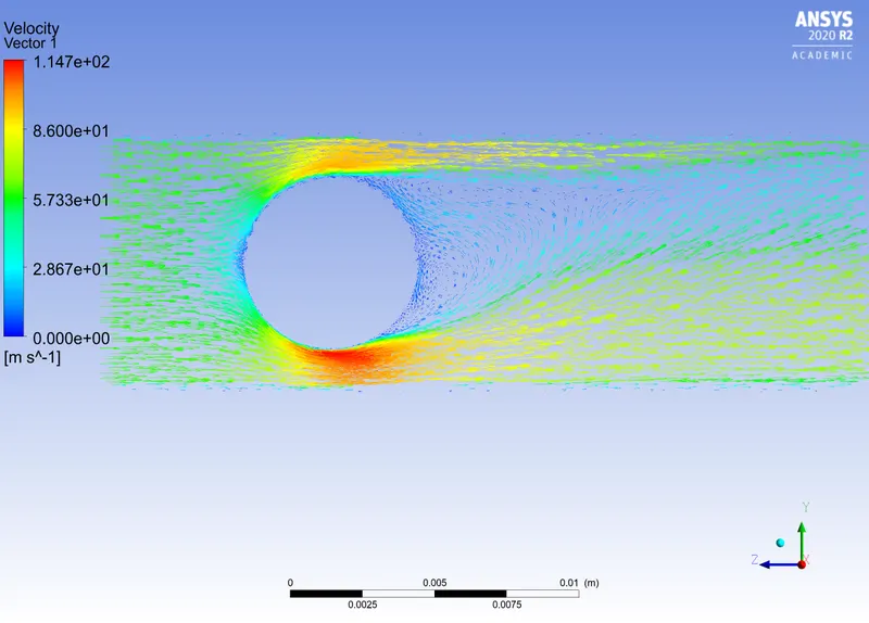
2. For the below geometry performs a 3D simulation and explain the recirculation region using velocity vectors.
3. Consider the flow direction of air, the ball is traveling opposite to it at 60m/s. Explain in which direction the ball will curve by visualizing the wake region.

Solution:

1) Literature Review on Various turbulence models in modern engineering applications:

Spalart–Allmaras (S–A):

The Spalart–Allmaras model is a one-equation model that solves a modeled transport equation for the kinematic eddy turbulent viscosity. The Spalart–Allmaras model was designed specifically for aerospace applications involving wall-bounded flows and has been shown to give good results for boundary layers subjected to adverse pressure gradients. It is also gaining popularity in turbomachinery applications.

k–ε (k–epsilon):

K-epsilon (k-ε) turbulence model is the most common model used in computational fluid dynamics (CFD) to simulate mean flow characteristics for turbulent flow conditions. It is a two-equation model which gives a general description of turbulence by means of two transport equations (PDEs). The original impetus for the K-epsilon model was to improve the mixing-length model, as well as to find an alternative to algebraically prescribing turbulent length scales in moderate to high complexity flows.

k–ω (k–omega):

In computational fluid dynamics, the k–omega (k–ω) turbulence models a common two-equation turbulence model that is used as a closure for the Reynolds-averaged Navier–Stokes equations (RANS equations). The model attempts to predict turbulence by two partial differential equations for two variables, k, and ω, with the first variable being the turbulence kinetic energy (k) while the second (ω) is the specific rate of dissipation (of the turbulence kinetic energy k into internal thermal energy).

SST (Menter’s Shear Stress Transport):

SST (Menter's shear stress transport) turbulence model is a widely used and robust two-equation eddy-viscosity turbulence model used in computational fluid dynamics. The model combines the k-omega turbulence model and K-epsilon turbulence model such that the k-omega is used in the inner region of the boundary layer and switches to the k-epsilon in the free shear flow.

Reynolds stress equation model

The Reynolds stress equation model (RSM), also referred to as the second-moment closure model, is the most complete classical turbulence modeling approach. Popular eddy-viscosity-based models like the k–ε (k–epsilon) model and the k–ω (k–omega) models have significant shortcomings in complex engineering flows. This arises due to the use of the eddy-viscosity hypothesis in its formulation. For instance, inflows with high degrees of anisotropy, significant streamline curvature, flow separation, zones of recirculating flow, or flows influenced by rotational effects, the performance of such models is unsatisfactory. In such flows, Reynolds stress equation models offer much better accuracy.

Eddy viscosity-based closures cannot account for the return to isotropy of turbulence, observed in decaying turbulent flows. Eddy-viscosity-based models cannot replicate the behavior of turbulent flows in the Rapid Distortion limit, where the turbulent flow essentially behaves like an elastic medium.

• We cannot use DNS because it generates a mesh that is very small and tries to capture all anomalies(cells), so as the mesh cells increase the time taken to solve will increase. Due to this industries don't prefer this method.

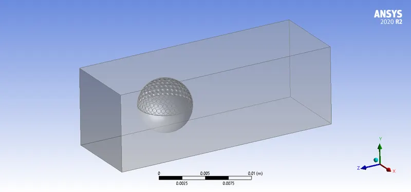
2) To do a 3D simulation of a golf ball and explain the recirculation region when the ball is traveling at 60m/s.

3D CAD model of the given geometry:

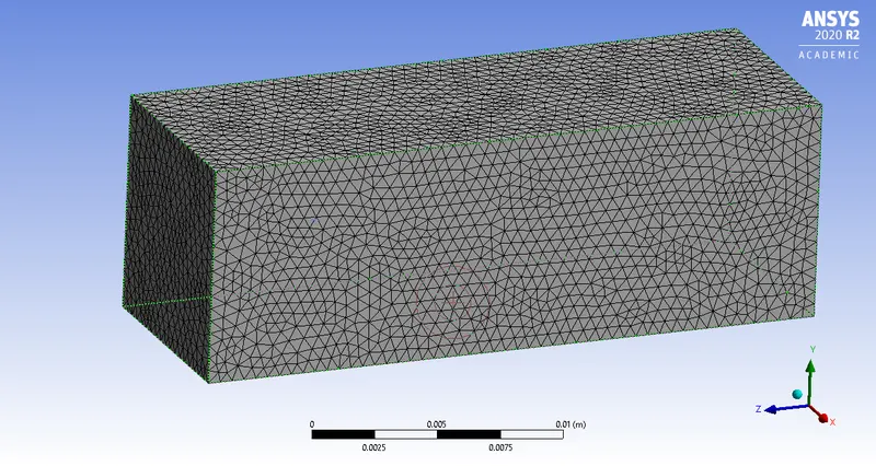
Meshing:

Mesh Size 0.5mm:

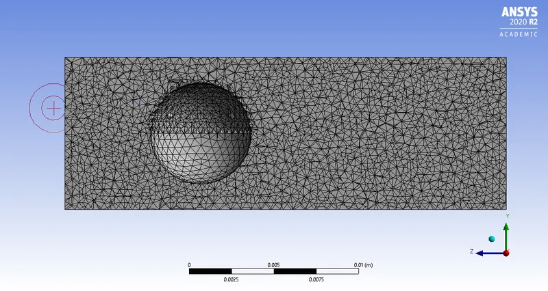
Cross Section of the Mesh:

Results:

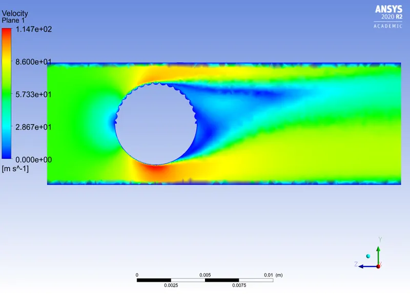
(i) Velocity Contour:

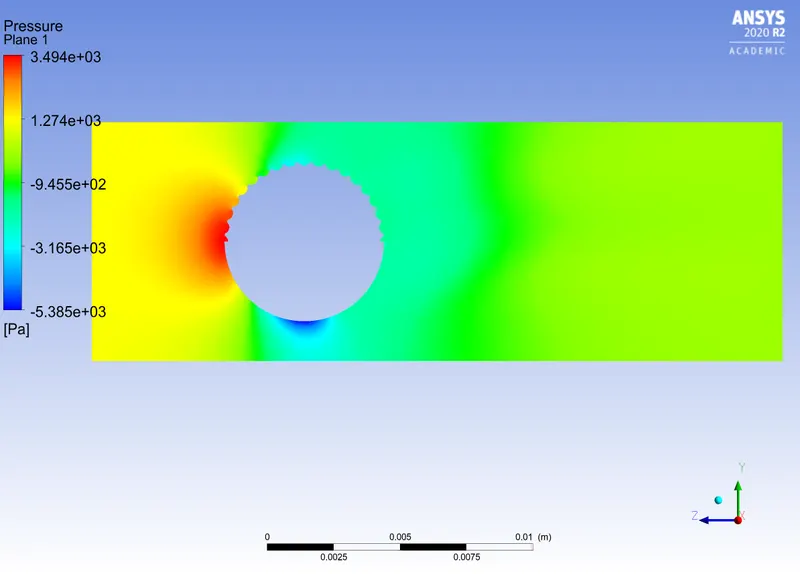
(ii) Pressure Contour:

(iii) Velocity Vector Plane:

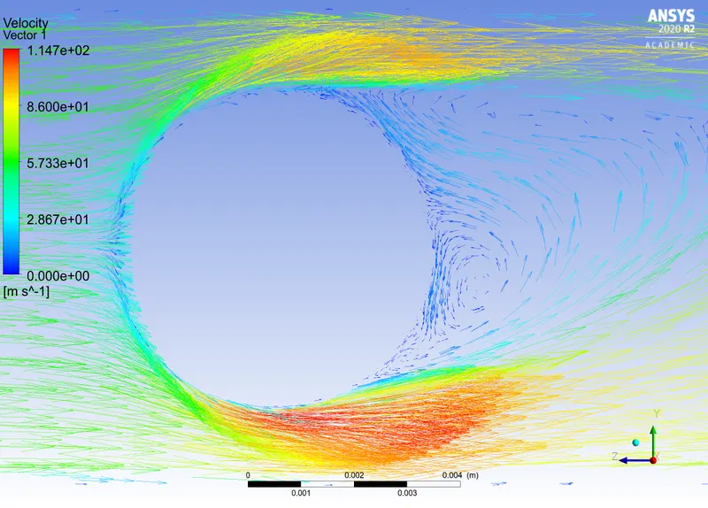
3) Explain in which direction the ball will curve by visualizing the wake region.

1. By inspecting the velocity vectors we can determine the direction of the ball and say it's going down.
2. The dimples on the golf ball help to reduce the drag by reducing the wake region (recirculation).
3. It also helps the flow to be attached and tries to separate the flow away from the golf ball.