Week 5 - Rayleigh Taylor Instability

AIM

To perform the Rayleigh Taylor Instability simulation and study the affects of Atwood number value on the behaviour of the instability using ANSYS Fluent.

INTRODUCTION

Rayleigh Taylor Instability is one of the best example for hydrodynamic instability. This phenomenon was first introduced by Lord Rayleigh and later it was observed for all accelerated fluids by G.I Taylor . Study of this instability phenomenon is relevant in understanding the behaviour of mushroom clouds formed after volcanic eruptions or nuclear explosions , instabilities in plasma fusion reactors and even in astrophysics & electrohydrodynamics(EHD).

OBJECTIVE

1. To perform the simulation for two different mesh sizes and to compare the results by showing the animations.
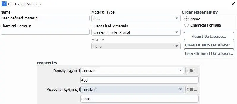
2. To create a user defined material with density 400 `(Kg)/m^3` & viscosity 0.001 `(Kg)/(ms)` and to perform the simulation for refined mesh.

THEORY

Rayleigh Taylor Instability is an instability of an interface between two fluids of different densities when the heavier fluid lies above the lighter fluid in a gravitational field.

This phenomenon is shown in the diagram given below,

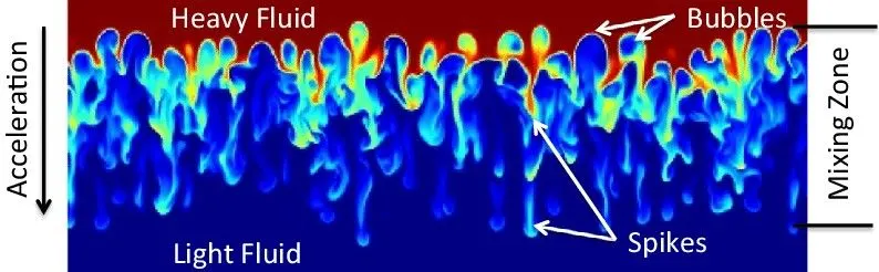
A common example for this instability is water on top of oil. In this case when the interface is disturbed , the hydrostatic pressure is generated causing the heavier fluid to move downwards and to mix with the lighter fluid. The amplitude of perturbation initially will grow exponentially and after some time it saturates.

It was observed that for small density differences the interface rolls up into two counter-rotating vortices and for large density differences the heavy fluid falls in smooth, pointed spikes into the light fluid, while the light fluid forms big rounded bubbles that propagate into the heavy fluid.

A dimensionless number called Atwood number is used in the study of hydrodynamic instabilities. It is a dimensionless density ratio defined as ,

`A = (rho_1-rho_2)/(rho_1+rho_2)`

Where , `rho_1` is the density of the heavier fluid and `rho_2` is the density of the lighter fluid.

If the value of Atwood number is closer to `1` , then the light fluid flows into the heavy fluid in the form of round topped bubbles with circular cross sections. If it is closer to `0` , then we would find patterns of interpenetrating bubbles.

Types of instabilities

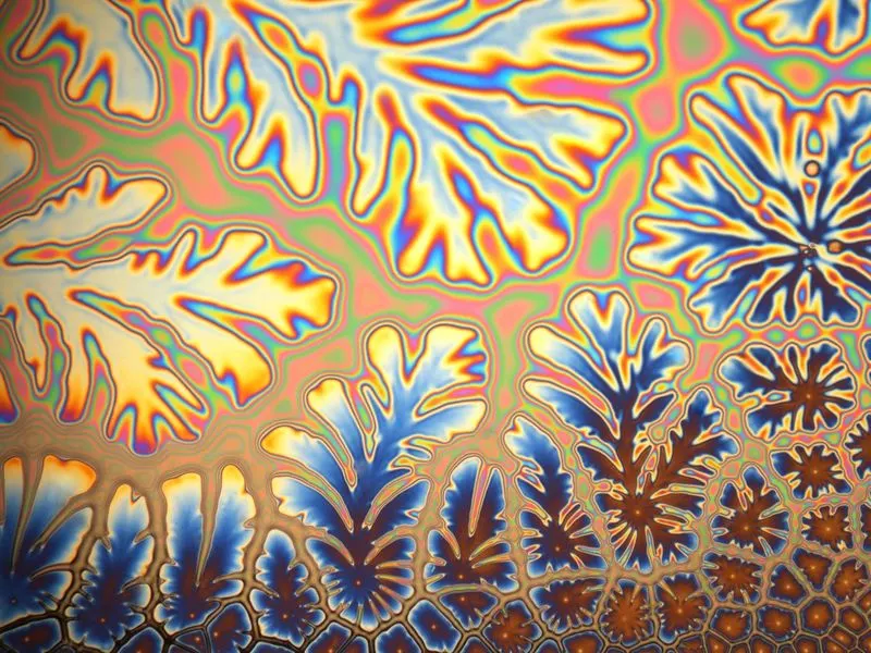
• Saffman_Taylor instability :- This is also known as viscous fingering and in this type of instability patterns are formed in a morphologically unstable interface between two fluids in a porous medium. This type was mathematically decribed by Phillip Saffman and G.I Taylor. It occurs when less viscous fluid displaces more viscous fluid. This instability pattern is shown below,

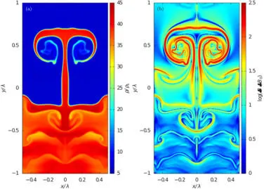
• Richtmyer–Meshkov instability:- This type of instability occurs when two fluids of different density are impulsively accelerated. Such impulsive accelerations are caused by the passage of a shock wave. This instability can be considered the impulsive-acceleration limit of the Rayleigh–Taylor instability.

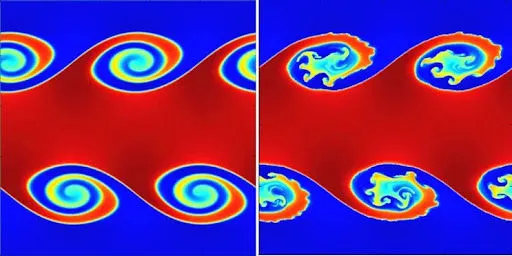
• Kelvin-Helmholtz instability :- It occurs when there is velocity shear in a single continuous fluid or when there is a velocity difference across the interface between two fluids.

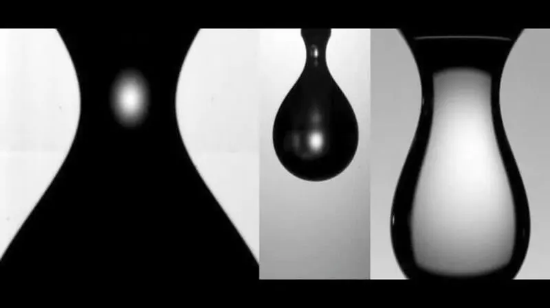
• Plateau-Rayleigh instability :- This instability explains the phenomenon of breaking up of falling stream of fluid into smaller packet with the same volume but less surface area. It is caused due to the surface tensions of the liquids by which it tends to minimize their surface area.

 

PROCEDURE

• To set up the geometry space claim software is used. The 2-D geometry created using this software is shown below ,

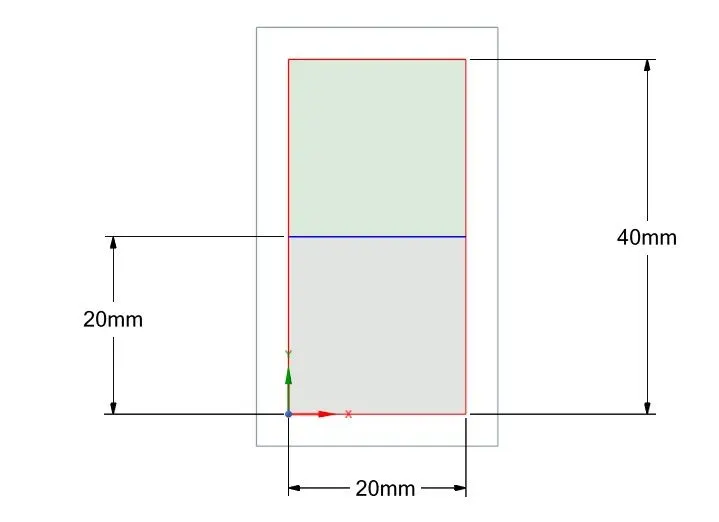
• The surface is created using the pull tool and share topology tool has been used to get conformal mesh.
• To mesh this geometry ANSYS meshing software is used.
• A coarse mesh and a refined mesh is made. The element size for coarse mesh is `0.5mm` and that refined mesh is `0.25mm`.

Coarse mesh ,

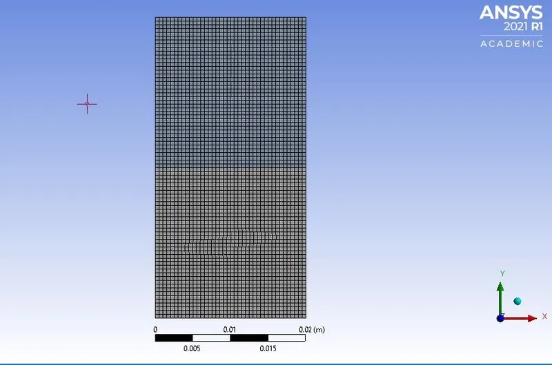
Number of cells in this mesh is 3200.

Refined mesh,

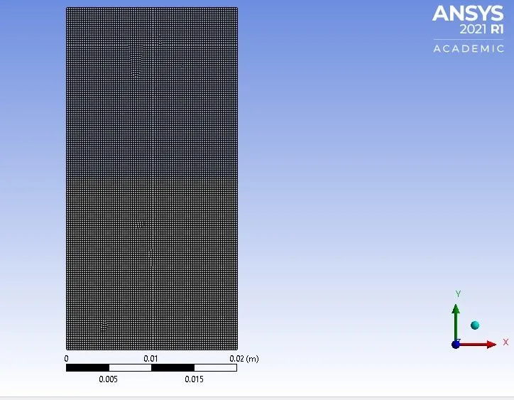
Number of cells in this mesh is 12800 and the refinement factor is 4 for this mesh.

SIMULATION SET-UP

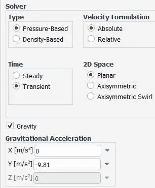
• Pressure based transient solver is used. Also the gravity setting is selected.

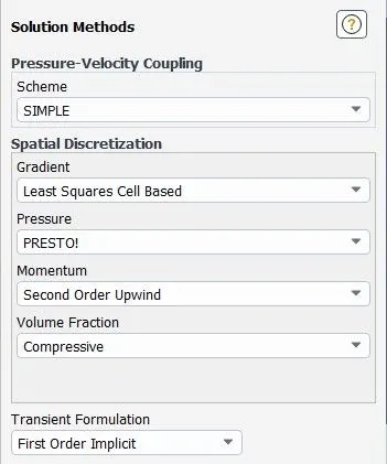
• The solution method used is SIMPLE with first order implicit transient formulation.

• For case 1 , materials used are default water and air.
• For case 2 , materials used are default water and user defined material shown below,

• Viscous model used is laminar.
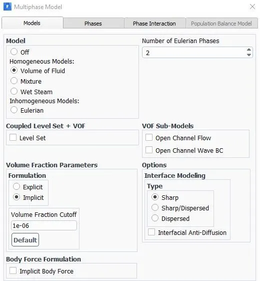
• Multiphase model used is Volume of fluid with 2 Eulerian phases and implicit formulation. Primary phase is defined as the lighter fluid and the secondary phase is defined as the heavier fluid.

• A contour is created for the phases of volume fraction.

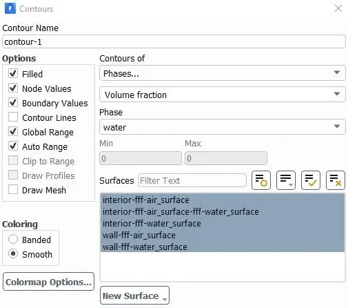
• Then the solution animation of this contour plot is made.

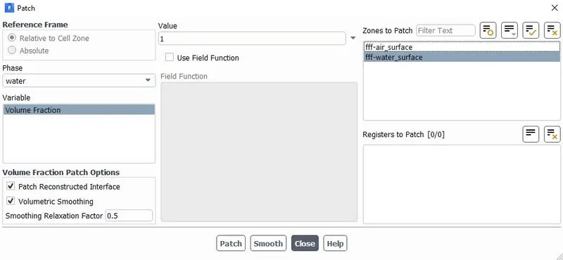
• After setting up the simulation parameters , standard initialization is done.
• Then the patching of the cells is done. Here the value of cell zone with water is given as 1 and for that of lighter fluid is given as 0.

RESULTS

• For coarse mesh with air and water as the fluids,

Animation :- https://drive.google.com/file/d/1G7v5WitlZSDhCvigOixewC-9ON14VBpT/view?usp=sharing

• For refined mesh with air and water as the fluids,

Animation :- https://drive.google.com/file/d/1ZlL-8WKbfP0fOjS-vhsV5Yt2BH5XpLh2/view?usp=sharing

• For refined mesh with user defined material and water as the fluids,

Animation :- https://drive.google.com/file/d/1G80qY-Xz9f2hNKH32FwHvU89rh2CkTCI/view?usp=sharing

CONCLUSION

The simulation of Rayleigh Taylor Instability has been done successfully using ANSYS software.

The simulations were done for two different mesh sizes and the results were analyzed. On decreasing the mesh size it was found that the simulation become much smoother and detailed. The step size used was smaller in case of refined mesh.

Also the simulations were carried out using transient solvers as the time step size required to capture the instabilities is very low and it is only possible using a transient solver. These instabilities are time dependent and hence the results will be accurate if the solver used is transient.

The Atwood number when the fluids used were air and water was found out to be `0.99`. In case of user defined material of density `400 (Kg)/m^3` and water it was found out to be `0.42`.

From the animations it could be seen that , in case of higher Atwood number the bubbles formed are larger like plumes and the amplitude of the disturbances are also high. This is due to the fact that higher the density ratio stronger the force to cause interface instability. Also the settling time is lower at higher Atwood number.

Where as in case of smaller Atwood number the bubbles formed were of smaller size and the settling time is higher. Also the amplitude of disturbances are smaller in this case.