Design of an Electric Vehicle

AIM

To create a MATLAB model of an electric car which uses a battery and a DC motor, by choosing suitable blocks from Powertrain block set.

THEORY

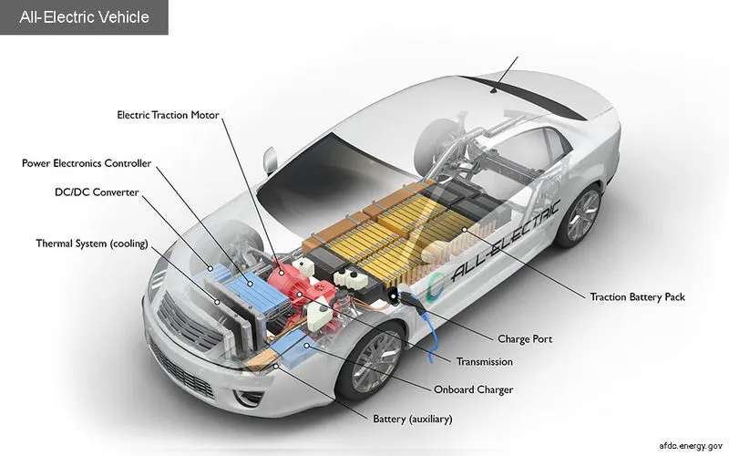
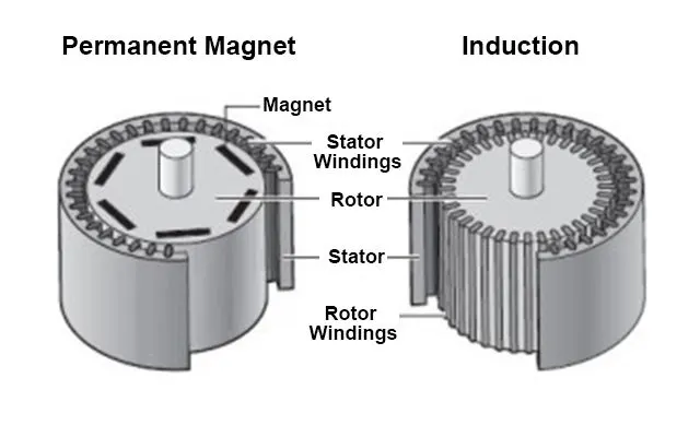
An electric car is a vehicle that is propelled by one or more electric motors, using energy stored in rechargeable battery packs. These are eco-friendly and has higher efficiency compared to ICE cars. An electric vehicle is 69-72% efficient when counted against stored chemical energy and around 59-62% efficient when counted against required energy to recharge. They use electric motors for propulsion. The most common types of motors used are Permanent Magnet Synchronous Motor (PMSM) and three phase induction motor.

Motor comparison,

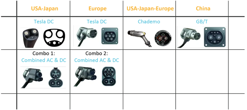
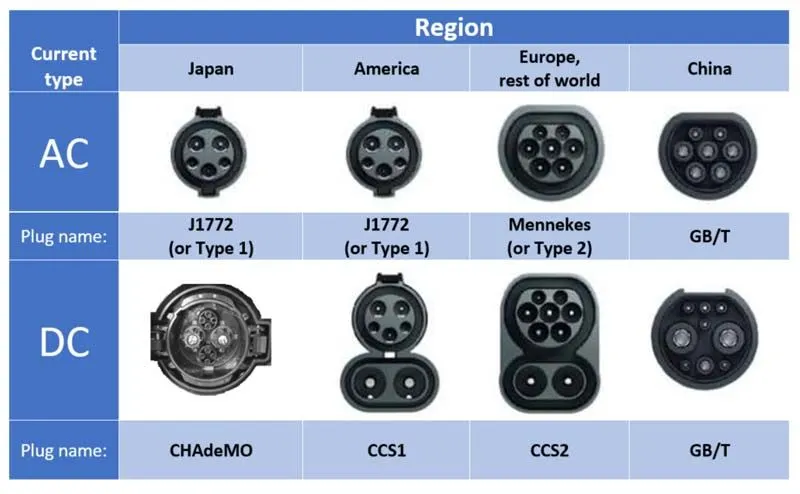
The battery packs are recharged using AC/DC charging technologies. AC charging is slow as it has to be converted to DC. Hence for fast charging DC chargers are used. The charging sockets has different standards as shown below,

BLOCK DIAGRAM

The block diagram for an Electric vehicle which uses a battery and a DC motor is shown below,

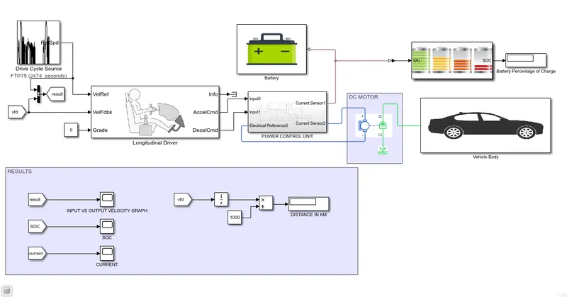
Now let us look at each of the blocks used to create this MATLAB model.

• Drive cycle data

For this we have used Drive cycle source block.

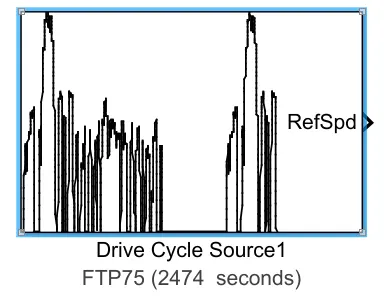
The block parameters for this block is as shown below,

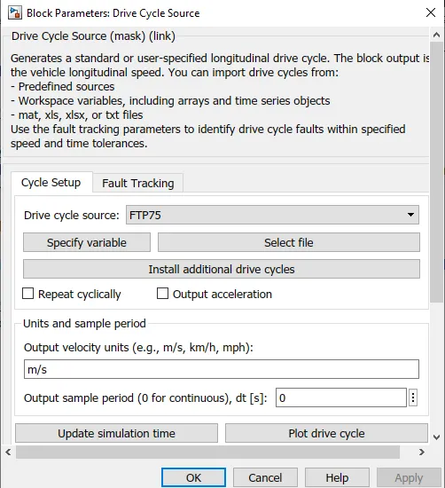
This block will help us in inputting the drive cycle data , whether it is built in or custom made by the user. That is we can use custom made drive cycle data in excel sheet using this block.

For this model we have used FTP 75 drive cycle , which is built-in in this block.

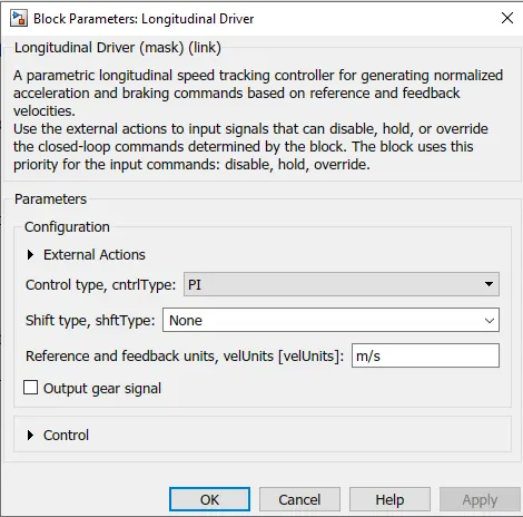
• Longitudinal driver

This block is used to create a longitudinal speed-tracking controller and it is based on reference and feedback velocities, the block generates normalized acceleration and braking commands that can vary from 0 through 1. We can use this block to model the dynamic response of a driver or to generate the commands necessary to track a longitudinal drive cycle.

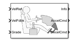
The block parameters is as shown below,

• Power control unit subsystem

This subsystem has the blocks which are used to create the voltage signals to control the motor speed as per the input drive cycle data.

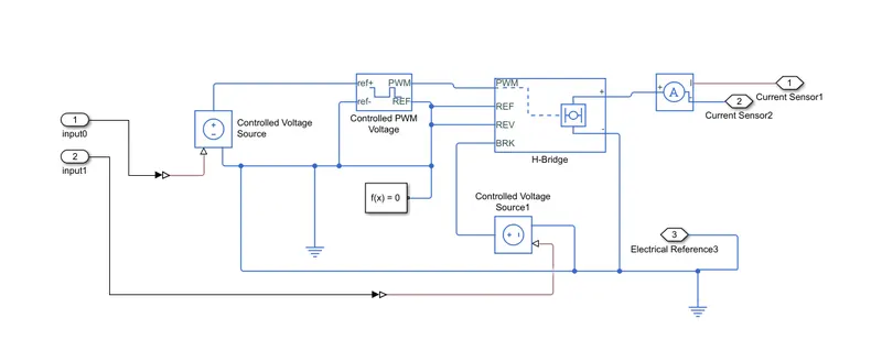
This subsystem is connected to the longitudinal driver block output ports namely acceleration command and deceleration command.

This subsystem will convert this acceleration and deceleration command into voltage signals using two controlled voltage source block, controlled PWM voltage block, a H-bridge and a current sensor.

• Controlled voltage source block

The block parameters is shown below,

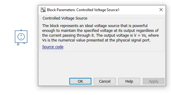
This block is used to maintain the specified voltage at its output regardless of the current flowing through the source.

• Controlled PWM voltage block

The block and its parameters is as shown below,

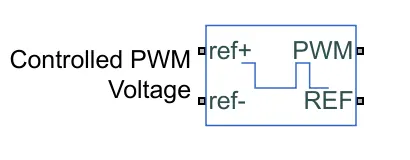
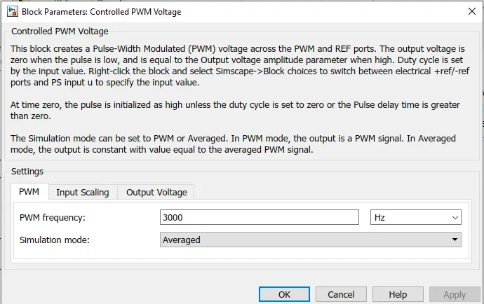
This block is used to create the pulse-width modulated (PWM) voltage.

Electrical input ports :- The block calculates the duty cycle based on the reference voltage across its ref+ and ref- ports. This modeling variant is the default.

The value of the Output voltage amplitude parameter determines amplitude of the output voltage.

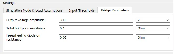
• H-bridge block

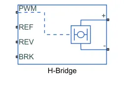
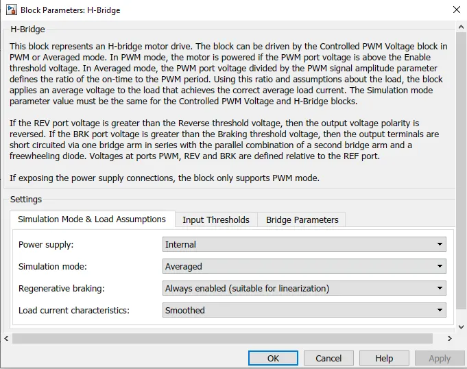
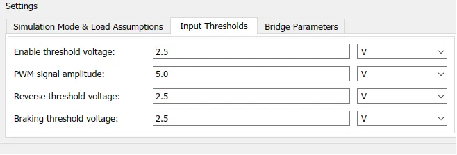
This block is used to change the polarity of the voltage applied across the DC motor so as to run the motor in forward and reverse direction as per the input command.

The block and its parameters are shown below,

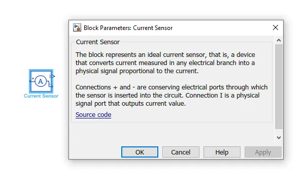
• Current sensor block

This is used to measure the current flowing through the H-bridge.

The block and its parameters is shown below,

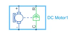
• DC motor

To convert the electrical energy to mechanical energy we use motors. In this electric vehicle model we have used DC motor. This motor can act as a generator also in case of regenerative braking.

The motor block and its parameters are shown below,

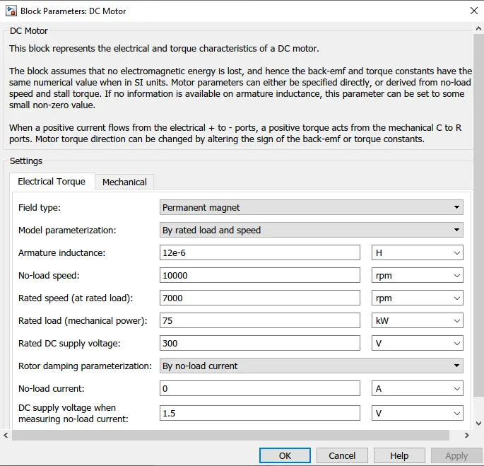
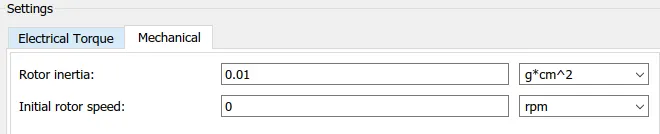
This block represents the electrical and torque characteristics of a DC motor.

• Battery subsystem

In this subsystem we have a battery block , a controlled current source block and a goto block.

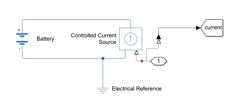
• Battery block

This battery block represents a simple battery model. The block models the battery as a series internal resistance and a constant voltage source.

The block and its parameters are shown below,

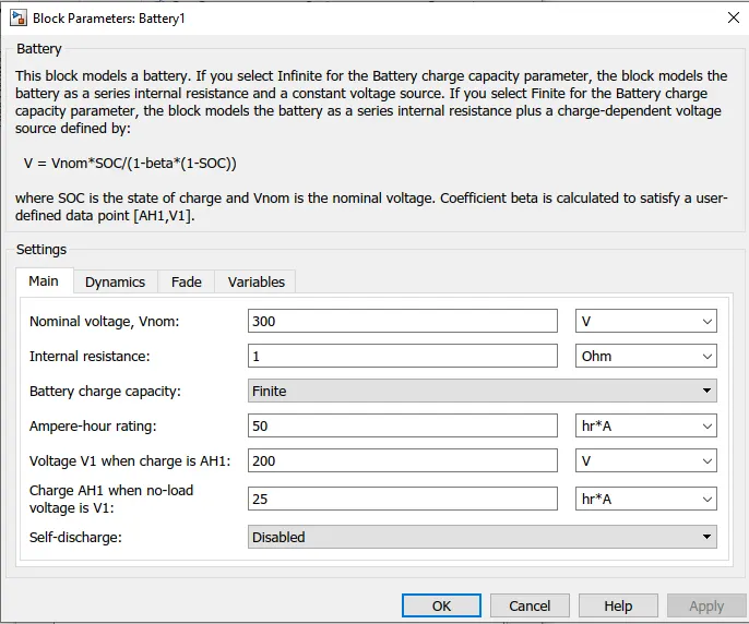
All other parameter sections are kept at default values.

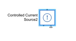
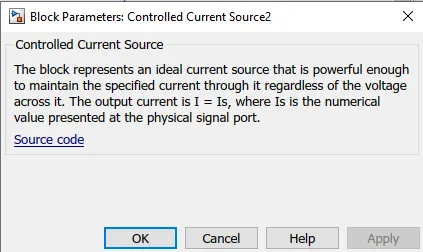
• Controlled current source block

This block gives a constant current output regardless of the voltage across it.

The block and its parameters are shown below,

• Goto block

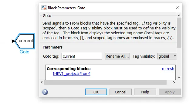
It is used to pass values to the ‘From block’ so that this value can be accessed from anywhere in the Simulink diagram. This input can be a real or complex valued signal or vector of any data type. This ‘From block’ and ‘Goto block’ allows us to pass a signal from one block to another without actually connecting them.

The block diagram & parameters of Goto block is shown below,

• State of charge calculation subsystem

The block diagram of the subsystem is as shown below,

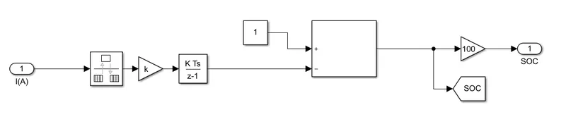
The input for this is from the current sensor.

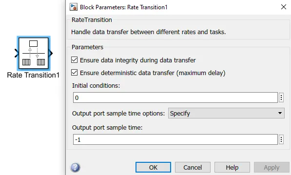
Now this is connected to the rate transition block. This handles the transfer of data between blocks operating at different rates. The block and its parameters are shown below,

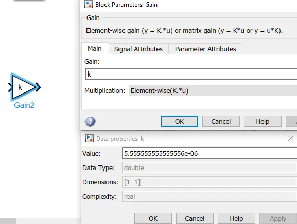
Then a gain block is connected to it. This gain will multiply the value of `k= 1/(A*sec)` , where `A*sec` is the ampere second value of the battery.

In this case the battery capacity is in `A*hr` , which is ampere hour.

To convert ,

`A*sec = A*hr *(3600)`

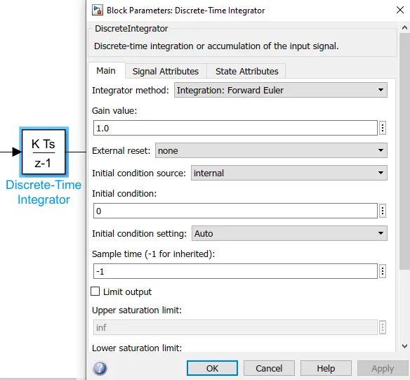
Then to add all these values with respect to time , we have used a Discrete-time integrator. This block will accumulate the input signal. The block and its parameters are shown below,

Now this summed value is subtracted from 1 , which will give us the remaining State Of Charge . To convert this to percentage , we have multiplied by 100 using another gain block.

Also a Goto block is used here to get SOC values.

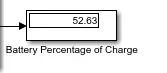
The output from this subsystem is connected to a displaye block , which will display the Battery Percentage as shown below,

• Vehicle body subsystem

This subsystem represents the body of a vehicle. The block diagram for this subsystem is shown below,

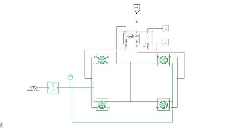
The input to this subsystem is the mechanical rotational conserving port of the DC motor block.

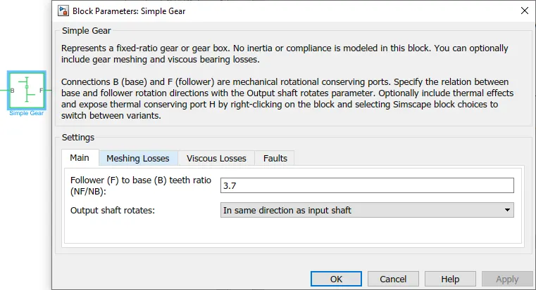
This is connected to the single speed gear box of gear ratio 3.7. This block and its parameters are shown below,

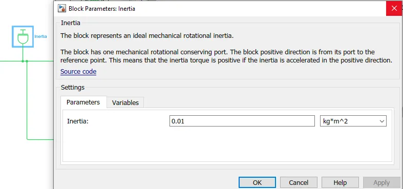
The inertia acting on the shafts is given using a Inertia block. This block and its parameters are shown below,

Now the simple gear is connected to all four wheels , representing an All wheel Drive vehicle. The tires are represented using tire (magic formula) block. This block and its parameters are shown below,

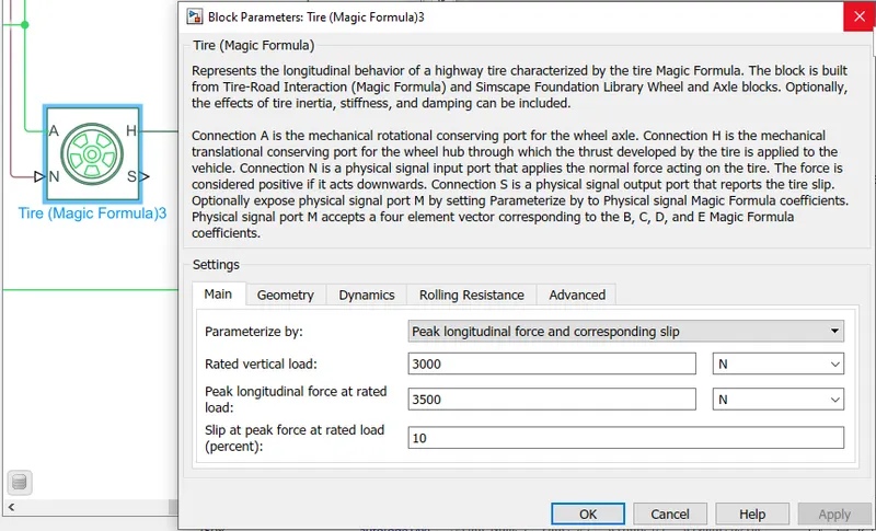
The simple gear is connected to the axle port of the tire block.

Now to represent the vehicle body we have used the vehicle body block . This block and its parameters are shown below,

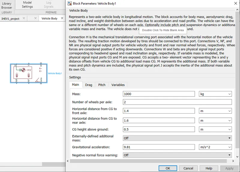
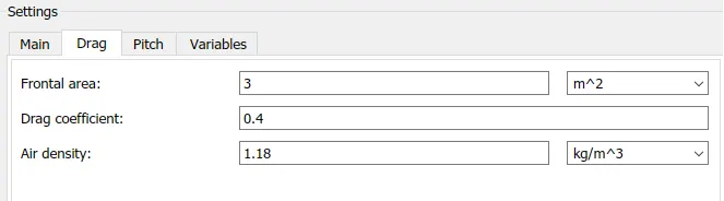
Now to the front and rear normal forces ports represented by NF & NR respectively of the vehicle body we have connected the four tire. Two at NF and two at NR ports. This represents the front 2 tires and the rear 2 tires.

Also the mechanical translational conserving port for the wheel hub represented by ‘H’ in tire block is connected to the port ‘H’ in the vehicle body block which represents the mechanical translational conserving port associated with the horizontal motion of the vehicle body.

To the gradient and wind speed ports of the vehicle body block , we have connected physical signal constant block.

The output from the vehicle body is the velocity of the vehicle in m/s. This output is connected to the Goto block with tag ‘vfd’.

Now coming back to the longitudinal driver block, the VelFdbk input to this block is given using the ‘From block ‘ with tag ‘vfd’. This is the output from the vehicle body block.

RESULT

The results section of this EV model is shown below,

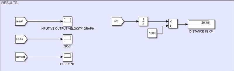
Here the first scope is input vs output velocity graph. This scope has two inputs , one is FTP 75 drive cycle and the other one is the velocity feedback. This two is combined using a bus and connected to a Goto block with tag ‘result’ and the corresponding ‘From block’ is connected to the scope to get this graph.

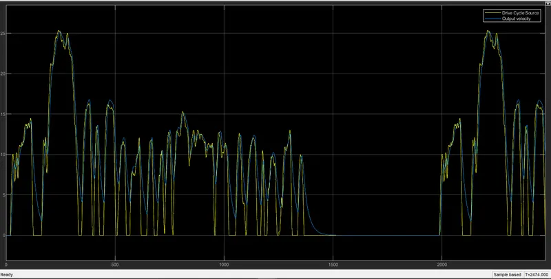
The resulting graph for this scope is shown below ,

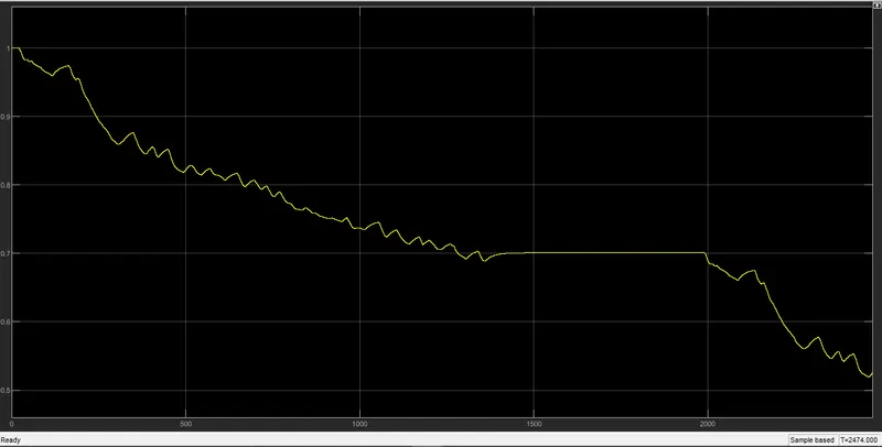
The next scope is used to get the change in SOC value with respect to time. The input for this scope is ‘From block’ with tag ‘SOC’.

The resulting graph is shown below,

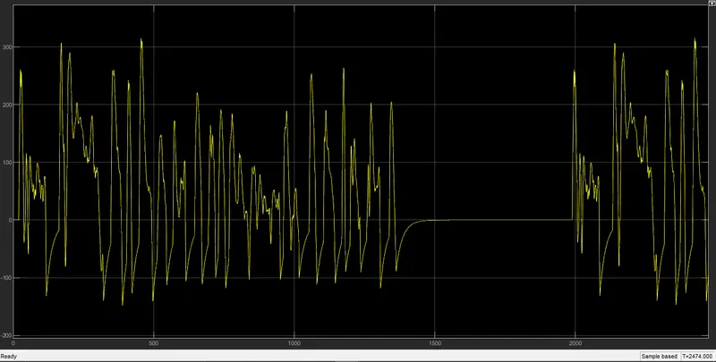
The third scope is used to get the current value with respect to time. Its input is ‘From block’ with tag ‘current’.the resulting graph is shown below,

The last result displays the distance covered by the vehicle in Km. It is calculated by integrating the velocity feedback value and dividing it by 1000 to convert it to Km.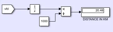

CONCLUSION

The MATLAB model of an electric car which uses a battery and a DC motor has been successfully made by choosing suitable blocks from Powertrain block set and following conclusions has been drawn from the results.

From the input vs output velocity graph we can see that the EV model that we designed have traced the FTP 75 drive cycle very closely. Only when the speed suddenly drops to 0 in the FTP 75 drive cycle , the model takes time to catch up. On all other occasions the model traced the drive cycle closely.

Now looking at the SOC graph we can see that almost 50% of the battery capacity is used for completing this drive cycle. And also we can see sudden spikes in that graph , these spikes represents the regenerative braking region. During which the SOC value increases.

And from the Current variation graph , we can see that the maximum current value during normal driving is around 300A and during regenerative braking the maximum current value reached is near to 150A.

The distance covered is 20.48 Km which is higher than the drive cycle data. For FTP 75 the total distance is 17.77Km. But still the value is closer to that FTP 75 value , showing that the model is quite accurate in following the drive cycle data.