Week 3.5 - Deriving 4th order approximation of a 2nd order derivative using Taylor Table method

AIM

A. Derive the following 4th order approximations of the second-order derivative,

1. Central difference
2. Skewed right-sided difference
3. Skewed left-sided difference

B. To write a program in Matlab to evaluate the second-order derivative of the analytical function `exp(x)*cos(x)` and compare it with the 3 numerical approximations derived.

C. To describe why a skewed scheme is useful and what can a skewed scheme do that a central difference scheme cannot.

THEORY

We have three different methods to approximate a given derivative. They are explained below,

Central difference method

In this method the numerical stencil is symmetric , i.e same number of nodes will be present on either side of the starting node. This method gives much more accurate results compared to other two methods.

Skewed right-sided difference

In this method the numerical stencil is not symmetric and hence the name skewed. In this method the grid points are taken only on the right side of the starting known point. This method is not as accurate as compared to central difference method.

Skewed left-sided difference

This method is also not symmetric , since the nodes are taken only on the left side of the initial point. The accuracy of this method is comparable to that of right-sided method and it is always better than right-sided point at any given value of step size. But this difference is very small and hence we can say both left and right sided methods are equally accurate.

For finding the coefficients of the difference equation we have used Taylor table method. This is a general method for choosing the coefficients of a finite difference formula to ensure the highest possible order of accuracy.

This table is based on the Taylor series equation and its coefficients. The standard equation for Taylor series is given below,

`sum_(n=0)^infty(f^n(x))/(n!)(Deltax)^n`

Where , `f^n(x)` is n^th derivative of the function ‘`f`’ at point ‘`x`’ , `Deltax` is the step size

OBJECTIVE

1. To prove that the skewed schemes are fourth-order accurate.
2. To plot a graph that compares the absolute error between the three methods of approximations.

CALCULATION

Derivation of central difference method

The formula for finding the 4^th order approximation of a second derivative using central difference method is as follows,

`(delta^2f)/(deltax^2) approx (a*f(x-2Deltax)+b*f(x-Deltax)+c*f(x)+d*f(x+Deltax)+e*f(x+2Deltax))/(Deltax^2)` ---Eq(1)

Here , `f` is the function whose second derivative has to be found out , `Deltax` is the step size and `x` is the initial value.

Now to solve this we have to find the values of the 5 coefficients , namely a,b,c,d & e.

To do this , first we have to expand each terms using Taylor series and solve for these coefficient. But this method is time consuming ans so instead we use Taylor table method. In this method , we won’t expand each terms in the above equation individually. Instead a table will be drawn in which the columns will represent the order of derivative and rows will represents the terms whose Taylor series expansion has to be found out. And then the coefficients will written in the respective places.

Taylor table for the above equation is shown below,

	ORDER OF DERIVATIVE
TERMS	`f(i)`	`Deltaxf^I(x)`	`Deltax^2f^(II)(x)`	`Deltax^3f^(III)(x)`	`Deltax^4f^(IV)(x)`
`a*f(i-2)`	`a`	`-2a`	`(4/2)a`	`(-8)/6a`	`16/24a`
`b*f(i-1)`	`b`	`-b`	`b/2`	`-b/6`	`b/24`
`c*f(i)`	`c`	`0`	`0`	`0`	`0`
`d*f(i+1)`	`d`	`d`	`d/2`	`d/6`	`d/24`
`e*f(i+2)`	`e`	`2e`	`(4/2)e`	`8/6e`	`16/24e`
Coefficient sum value	`0`	`0`	`1`	`0`	`0`

Here we can see that the sum of coefficients in the 3^rd column is 1. This is because we are finding the value of second derivative.

Next step is to find the value of the coefficients by putting this in a matrix. Row of this matrix contains the column of the above table and the column of this matrix contains row of the above table.

The matrix is given below,

`A=[[1,1,1,1,1] , [-2 ,-1 ,0, 1, 2] , [2, 1/2, 0 ,1/2, 2] , [-8/6, -1/6 ,0 ,1/6 ,8/6] , [16/24, 1/24, 0, 1/24, 16/24]]`

Now we will create a matrix containing variables as shown below,

`B = [[a],[b],[c],[d],[e]]`

And the last matrix is sum of coefficients matrix , which is given below,

`X = [[0],[0],[1],[0],[0]]`

As we know that the value of `A*B=X`

Equating this we can find the value of the coefficients. After finding the coefficients we will put those in the Eq (1).

Derivation of skewed right-sided difference method

The formula for finding the 4^th order approximation of a second derivative is as follows,

`(delta^2f)/(deltax^2) approx (a*f(x)+b*f(x+Deltax)+c*f(x+2Deltax)+d*f(x+3Deltax)+e*f(x+4Deltax)+g*f(x+5Deltax))/(Deltax^2)` ---Eq(2)

Taylor table for the above equation is shown below,

	ORDER OF DERIVATIVE
TERMS	`f(i)`	`Deltaxf^I(x)`	`Deltax^2f^(II)(x)`	`Deltax^3f^(III)(x)`	`Deltax^4f^(IV)(x)`	`Deltax^4f^(V)(x)`
`a*f(i)`	`a`	`0`	`0`	`0`	`0`	`0`
`b*f(i+1)`	`b`	`b`	`b/2`	`b/6`	`b/24`	`b/120`
`c*f(i+2)`	`c`	`2c`	`4/2c`	`8/6c`	`16/24c`	`32/120c`
`d*f(i+3)`	`d`	`3d`	`9/2d`	`27/6d`	`81/24d`	`243/120d`
`e*f(i+4)`	`e`	`4e`	`16/2e`	`64/6e`	`256/24e`	`1024/120e`
`g*f(i+5)`	`g`	`5g`	`25/2g`	`125/6g`	`625/24g`	`3125/120g`
Coefficient sum value	`0`	`0`	`1`	`0`	`0`	`0`

Matrix `A = [[1,1,1,1,1,1] , [0 ,1 ,2 ,3 ,4, 5] ,[0, 1/2 ,2, 9/2, 8 ,25/2], [0 ,1/6 ,4/3, 9/2, 32/3, 125/6] , [0 ,1/24, 16/24, 81/24, 256/24 ,625/24] , [0 ,1/120, 32/120 ,243/120, 1024/120, 3125/120]]`

Matrix `B = [[a],[b],[c],[d],[e],[g]]`

And `matrix C = [[0],[0],[1],[0],[0],[0]]`

Now putting these in the below equation,

`A*B=X` , we get the values of the coefficients.

After finding the coefficients we will put those in the equation (2).

Derivation of skewed left-sided difference method

The formula for finding the 4^th order approximation of a second derivative is as follows,

`(delta^2f)/(deltax^2) approx (a*f(x-5Deltax)+b*f(x-4Deltax)+c*f(x-3Deltax)+d*f(x-2Deltax)+e*f(x-Deltax)+g*f(x))/(Deltax^2)` ---Eq(3)

Taylor table for the above equation is shown below,

	ORDER OF DERIVATIVES
TERMS	`f(i)`	`Deltaxf^I(x)`	`Deltax^2f^(II)(x)`	`Deltax^3f^(III)(x)`	`Deltax^4f^(IV)(x)`	`Deltax^4f^(V)(x)`
`a*f(i-5)`	`a`	`-5a`	`25/2a`	`-125/6a`	`625/24a`	`-3125/120a`
`b*f(i-4)`	`b`	`-4b`	`16/2b`	`-64/6b`	`256/24b`	`-1024/120b`
`c*f(i-3)`	`c`	`-3c`	`/2c`	`-27/6c`	`81/24c`	`-243/120c`
`d*f(i-2)`	`d`	`-2d`	`9/2d`	`-8/6d`	`16/24d`	`243/120d`
`e*f(i-1)`	`e`	`-e`	`4/2e`	`-1/6e`	`1/24e`	`-32/120e`
`g*f(i)`	`g`	`0`	`0`	`0`	`0`	`0`
Coefficient sum value	`0`	`0`	`1`	`0`	`0`	`0`

Matrix `A = [[1,1,1,1,1,1] , [-5 ,-4 ,-3 ,-2, -1, 0] , [25/2, 16/2, 9/2, 4/2 ,1/2, 0] , [-125/6, -64/6 ,-27/6 ,-8/6 ,-1/6 ,0] ,[625/24, 256/24, 81/24, 16/24, 1/24, 0], [-3125/120 ,-1024/120,-243/120, -32/120, -1/120, 0]]`

Matrix `B = [[a],[b],[c],[d],[e],[g]]`

And matrix `C = [[0],[0],[1],[0],[0],[0]]`

Now putting these in the below equation,

`A*B=X` , we get the values of the coefficients.

After finding the coefficients we will put those in the equation (3).

Order of accuracy

Now let us check whether the 2 skewed schemes are 4^th order accurate by using the following formula,

The order of accuracy, `P = N - Q`

Where N is the number of nodes in the stencil and Q is the order of derivative.

So from the above derivations , we know that order of derivative , `Q= 2`

And , `N= 6` , this is same as the number of coefficients in the equation.

So , `P = 6-2`

`= 4`

Hence its proved that the two skewed schemes are 4^th order accurate.

PROGRAM

This program will call functions containing the different methods of approximations calculation and will find the error for each methods of approximation at different values of dx. Also it will plot the graph between dx and error values of different methods of approximations. A comparison between analytical derivative and numerical approximations will also be done.

clear all
close all 
clc

%%

%defining variables
x=pi/3;
dx = linspace(pi/40,pi/4000,20);

%%

%calculating the exact value of second derivative of the given function
syms z;
f=exp(z)*cos(z);
%differentiating the function
f_2 = diff(f,2);
%exact value calculation
analytical_derivative = vpa(subs(f_2,z,pi/3));
%converting the symbolic variable to double precision
ad=double(analytical_derivative );

%%
 
% for loop to call the function and calculate for different values of dx
for i=1:length(dx)
    
cd(i) = central_differencing (x,dx(i));
rsd(i) = right_side_differencing (x,dx(i));
lsd(i) = left_side_differencing (x,dx(i));

%calculating the absolute error value
error_central_difference = abs(cd- analytical_derivative);
error_right_side_difference = abs(rsd- analytical_derivative);
error_left_side_difference = abs(lsd- analytical_derivative);

end

%%

%plotting the graphs 

% 1st graph
figure(1)
yline(ad,'--','LineWidth',2 ,'color','r');
hold on
plot(dx,cd,'color','k','LineWidth',2 );
hold on 
plot(dx,rsd,'color','g','LineWidth',2 );
hold on
plot(dx,lsd,'color','b','LineWidth',2 );
legend('analytical derivative','central differencing','right sided differencing','left sided differencing','location','best');
title('analytical derivative Vs other 3 differencing methods values')
ylabel('derivative value')
xlabel('dx value')

%2nd graph
figure(2)
loglog(dx,error_central_difference,'color','r','LineWidth',2 );
hold on
loglog(dx,error_right_side_difference,'color','g','LineWidth',2 );
hold on
loglog(dx,error_left_side_difference,'color','b','LineWidth',2 );
legend('central differencing error','right sided differencing error','left sided differencing error','location','best');
title('comparison of absolute error between 3 different  methods')
ylabel('error value')
xlabel('dx value')

• First we have defined the variables used for the calculations. Here we have used ‘linspace’ command to create equally spaced 20 values between pi/40 and pi/4000 for dx.
• Then the analytical value of the second derivative is calculated. For this we have used ‘diff’ command in MATLAB. This command will differentiate symbolic expressions or function.Syntax for this command is given below,

`"Df = diff(f,n)"` computes the n^th derivative of `f` with respect to the symbolic variable.

• For creating a symbolic variable we have used ‘syms’ command.
• After finding the second derivative of the given function we will substitute the value of the variable using ‘vpa’ command.
• This value will be stored as symbolic variable , so in order to convert we use ‘double’ command , which will convert it to double precision values.
• A for loop is opened with number of iterations equal to length of dx array.
• After that the functions are called inside the for loop. These functions contain the calculation for different methods of approximation.
• Then the error is calculated. Here we used ‘abs’ command , which will return the absolute value.
• Now the for loop is closed using the ‘end’ command.
• Next thing done is to plot a graph comparing the analytical derivative value with the values of other 3 differencing methods. To plot the analytical derivative value which is a constant value , we used ‘yline’ command. This command will plot a horizontal line with constant y-value.
• The second graph plots the comparison of absolute error between the three different methods. For plotting this we have used ‘loglog’ command to have better understanding of the characteristics.

FUNCTION PROGRAMS

Function to calculate central difference approximation is given below,

function [cd] = central_differencing (x,dx)

A=[1 1 1 1 1 ; -2 -1 0 1 2 ; 2 1/2 0 1/2 2 ; -8/6 -1/6 0 1/6 8/6 ; 16/24 1/24 0 1/24 16/24];
B= inv(A);
X=B(:,3);
a = X(1);
b = X(2);
c = X(3);
d=b;
e=a;

cd = (a*exp(x-(2.*dx)).*cos(x-(2.*dx))+b.*exp(x-dx).*cos(x-dx)+c*exp(x)*cos(x)+d.*exp(x+dx).*cos(x+dx)+e.*exp(x+(2*dx)).*cos(x+(2.*dx)))./dx.^2;
end

Function to calculate skewed right-sided difference approximation is given below,

function [rsd] = right_side_differencing (x,dx)

A=[1 1 1 1 1 1 ; 0 1 2 3 4 5 ; 0 1/2 2 9/2 8 25/2 ; 0 1/6 4/3 9/2 32/3 125/6 ; 0 1/24 16/24 81/24 256/24 625/24 ; 0 1/120 32/120 243/120 1024/120 3125/120 ];
B= inv(A);
X=B(:,3);
a = X(1);
b = X(2);
c = X(3);
d=X(4);
e=X(5);
g=X(6);

rsd = (a*exp(x)*cos(x)+b.*exp(x+dx).*cos(x+dx)+c.*exp(x+(2.*dx)).*cos(x+(2.*dx))+d.*exp(x+(3.*dx)).*cos(x+(3.*dx))+e.*exp(x+(4.*dx)).*cos(x+(4.*dx))+g.*exp(x+(5.*dx)).*cos(x+(5.*dx)))./dx.^2;
end

Function to calculate skewed left-sided difference approximation is given below,

function [lsd] = left_side_differencing (x,dx)

A=[1 1 1 1 1 1 ; -5 -4 -3 -2 -1 0 ; 25/2 16/2 9/2 4/2 1/2 0 ; -125/6 -64/6 -27/6 -8/6 -1/6 0 ; 625/24 256/24 81/24 16/24 1/24 0 ; -3125/120 -1024/120 -243/120 -32/120 -1/120 0 ];
B= inv(A);
X=B(:,3);
a = X(1);
b = X(2);
c = X(3);
d=X(4);
e=X(5);
g=X(6);

lsd = (a.*exp(x-(5.*dx)).*cos(x-(5.*dx))+b.*exp(x-(4.*dx)).*cos(x-(4.*dx))+c.*exp(x-(3.*dx)).*cos(x-(3.*dx))+d.*exp(x-(2.*dx)).*cos(x-(2.*dx))+e.*exp(x-dx).*cos(x-dx)+g*exp(x)*cos(x))./dx.^2;
end

• In all three of the functions, we have created the respective matrix containing the coefficients that we already derived.
• Then another matrix is created which is equal to the inverse of the first matrix. For this we have used the command ‘inv’ , which will find the inverse of a given matrix.
• Then the 3^rd column of this inverse matrix will be the required values of the coefficients. And we will assign each of this values to the respective coefficients and then use them in the equation.

These function programs will calculate the different methods of approximation as per the equations derived for them.

RESULTS

Let us look at the first plot showing the comparison between analytical and numerical values.

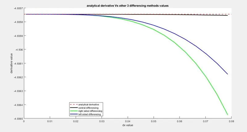
• Here we can see that the numerical derivative values are deviating from the analytical value as the step size increases. This shows that as we increase the step size the error also increases. Here the central differencing method is showing the least deviation and hence we can say that it is almost accurate at all values of dx in this case.
• Whereas right sided and left sided differencing methods are showing very large deviation from the exact value. This shows that these two methods are less accurate compared to central differencing method. Right sided method is the most deviating and hence it is the least accurate of all three methods.

Now let us look at the comparison of absolute error values of the three numerical approximation methods graph.

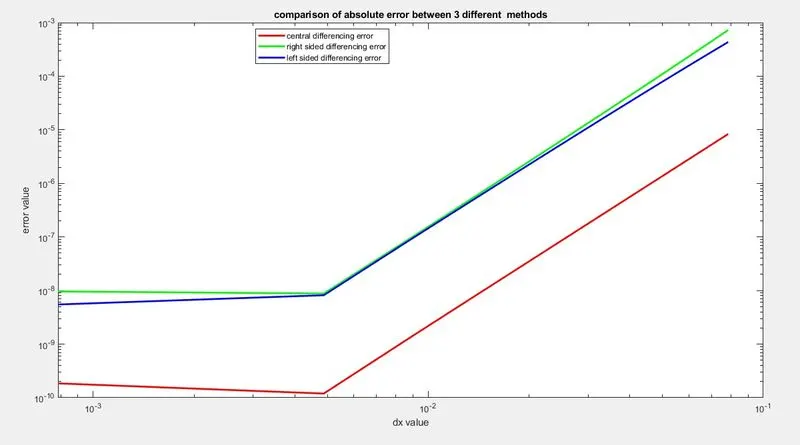
• In this graph we can see that the error is decreasing till a point as the value of dx is decreasing. At any given value of the dx we can see that the error value of central method is always lower compared to other two methods.
• Coming to the other two methods ,we can see that they are very close to each other , this means that the error values of these methods are comparable to each other and almost similar. Even then the left sided method is having low error at any given value of dx.

Now let us look at the part of this graph where the characteristics reverses , i.e the value of error starts increasing as the value of dx decreasing. This portion is shown below ,

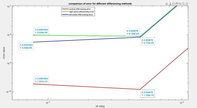
• Here we can see that the error is increasing for right sided method and central method , where as the left sided method is still decreasing but at a very slow rate.
• This is due to the introduction of round-off error to the calculation. A round-off error is the numerical error introduced after a repetitive number of calculations in which the computer is constantly rounding the number to some significant figure.
• When this happens the calculation will become unstable.

Advantage of skewed scheme over symmetric

To understand why a skewed is useful and what it can do that a symmetric can’t do , we need to take an example scenario , which is explained below,

Suppose if the flow field characteristics has to be evaluated starting from the boundary with second order accuracy. The y-axis is perpendicular to this boundary and we need to do the finite difference approximation at the boundary.

Let us first try to solve it using symmetric method , i.e central differencing , so for this method we need grid points on both sides of the initial point. So in this case we need to have values beyond the boundary , but this is not technically possible as there is no flow field beyond boundary. In this condition the symmetric method is of no use.

Now what are the other methods possible , we have forward differencing method which could be used but it is first order accurate , so we cannot use that.

Here comes the skewed schemes advantage. A skewed scheme is formulated by applying polynomial approach on Taylor series. In this example scenario we can apply skewed scheme because it uses information only on one side of the grid point at the boundary. So we need only the grid points above the boundary to find the finite difference expression for the derivative at the boundary. Also the order of accuracy can be decide as per the requirement by adding grid points.

CONCLUSION

MATLAB program that compares the central, right sided and left sided schemes of approximations for the second derivative against the analytical or exact derivative for a range of values for dx has been written successfully and the results has been plotted on a graph. Also the order of accuracy has been verified successfully.