Week 7 - Simulation of a 1D Super-sonic nozzle flow simulation using Macormack Method

AIM

To simulate the isentropic flow through a quasi 1D subsonic-supersonic nozzle using both the conservation form and non-conservation forms of governing equations solved with MacCormack's technique.

GOVERNING EQUATIONS

Integral form of the flow equations are as follows,

Continuity equation ,

`del/(delt)intintintrho*dv+intintrhoV*dS=0`

Momentum equation ,

`del/(delt)intintintrhou*dv+intintrhouV*dS=-intint(pdS)_x`

Energy equation,

`del/(delt)intintintrho(e+V^2/2)*dv+intintrho(e+V^2/2)V*dS=-intintpV*dS`

From these integral form of the governing flow equations we can derive the corresponding partial differential equations for both the conservation form and the non-conservation form.

For conservation form the partial differential equations are as follows,

Continuity equation ,

`(del(rhoA))/(delt)+(del(rhoAV))/(delx)=0`

Momentum equation ,

`(del(rhoVA))/(delt)+(del(rhoV^2A))/(delx)=-A(delp)/(delx)`

Energy equation,

`(del[rho(e+V^2/2)*A])/(delt)+(del[rho(e+V^2/2)V*A])/(delx)=-(del(pAV))/(delx)`

For non-conservation form the partial differential equations are as follows,

Continuity equation ,

`(del(rhoA))/(delt)+rhoA(delV)/(delx)+rhoV(delA)/(delx)+VA(delrho)/(delx)=0`

Momentum equation ,

`rho(delV)/(delt)+rhoV(delV)/(delx)=-R(rho(delT)/(delx)+T(delrho)/(delx))`

Energy equation,

`rhoC_v(delT)/(delt)+rhoVC_v(delT)/(delx)=-rhoRT((delV)/(delx)+V(del(ln A))/(delx))`

Where , `rho` is the density , `T` is the temperature , `V` is the fluid velocity , `A` is the area ,

`x` is the length , `t` is the time, `e` is the internal energy , `p` is the pressure , `C_v` is the specific heat at constant volume and `R` is the gas constant.

THEORY

A subsonic-supersonic nozzle considered here is one in which the flow expands isentropically to supersonic speeds from subsonic speeds. Here the inlet of the nozzle is considered to be from a reservoir whose cross-sectional area is considered to be infinity. The speed at the throat of the nozzle will be sonic , i.e mach number , M=1. At the exit of the nozzle the speed will be super sonic , i.e mach number , M>1.

This nozzle is shown below,

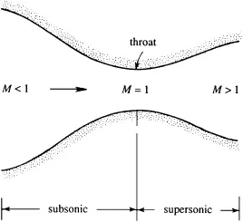
A quasi one-dimensional flow is defined as a flow whose properties across any given cross section is uniform , i.e the flow properties vary only with x-direction.

The governing equations for solving can be of two forms , namely conservation form and non-conservation form. In conservation form equation is derived from a flow model which is fixed in space. Whereas a non-conservation form equation is derived from a flow model moving with the fluid.

OBJECTIVE

• To plot the following graphs,

1. Steady-state distribution of primitive variables inside the nozzle
2. Time-wise variation of the primitive variables
3. Variation of Mass flow rate distribution inside the nozzle at different time steps during the time-marching process
4. Comparison of Normalized mass flow rate distributions of conservation form and non-conservation form.

• To perform a grid independence test on the solution.

DERIVATION

To solve the equations using MacCormack's technique we will change the governing equations for both conservation form and non-conservation form to non-dimensional form.

The flow variables in non-dimensional form is as follows,

Temperature , `T^' = T/T_0`

Density , `rho^' = rho/rho_0`

Length , `x^' = x/L`

Velocity , `V^' = V/a_0`

Time , `t^' = t/(L"/"a_0)`

Area , `A^' = A/A^"*"`

Where `T_0` , `rho_0` and `a_0` are the corresponding temperature, density and speed of sound in the reservoir. `L` is the length of the nozzle and `A^"*"` is the sonic throat area.

Now let us put these non-dimensional variables to the governing equations of both forms.

For non-conservation form the equations will become,

Continuity equation,

`(delrho^')/(delt^')=-rho^'(delV^')/(delx^')-rho^'V^'(del(lnA^'))/(delx^')-V^'(delrho^')/(delx^')`

Momentum equation ,

`rho^'(delV^')/(delt^')=-rho^'V^'(delV^')/(delx^')-(rho^'(delT^')/(delx^')+T^'(delrho^')/(delx^'))(RT_0)/(a_0^2)`

Here , `a_0 = sqrt(gammaRT_0)`

`(RT_0)/(a_0^2) = (gammaRT_0)/(gammaa_0^2)`

`= (a_0^2)/(gammaa_0^2)`

`= 1/gamma`

Where `gamma` is the ratio of specific heats.

Now the momentum equation becomes,

`(delV^')/(delt^')=-V^'(delV^')/(delx^')-(1/gamma)((delT^')/(delx^')+T^'/rho^'(delrho^')/(delx^'))`

Energy equation ,

`(delT^')/(delt^')=-V^'(delT^')/(delx^')-R/C_vT^'[(delV^')/(delx^')+V^'(del(ln A^'))/(delx^')]`

Here , `R/C_v = R/(R"/"(gamma-1))=gamma-1`

Now the energy equation becomes ,

`(delT^')/(delt^')=-V^'(delT^')/(delx^')-(gamma-1)T^'[(delV^')/(delx^')+V^'(del(ln A^'))/(delx^')]`

For conservation form the equations will become,

Continuity equation,

`(del(rho^'A^'))/(delt^')+(del(rho^'A^'V^'))/(delx^')=0`

Momentum equation ,

`(del(rho^'V^'A^'))/(delt^')+(del[rho^'V^('2)A^'+p^'A^'(p_0"/"(rho_0a_0^2))])/(delx^')=p^'(delA^')/(delx^')(p_0/(rho_0a_0^2))`

But here , `p_0/(rho_0a_0^2) = (p_0RT_0)/(rho_0a_0^2) = 1/gamma`

Hence the equation becomes,

`(del(rho^'V^'A^'))/(delt^')+(del[rho^'V^('2)A^'+(1"/"gamma)p^'A^'])/(delx^')=(1/gamma)p^'(delA^')/(delx^')`

Energy equation ,

`(del[rho^'(e^'/(gamma-1)+gamma/2V^('2))A^'])/(delt^')+(del[rho^'(e^'/(gamma-1)+gamma/2V^('2))V^'A^'+rho^'A^'V^'])/(delx^')=0`

PROCEDURE

Now let us use MacCormack's explicit technique to solve for the numerical solutions derived.

The grid point distribution is as shown below,

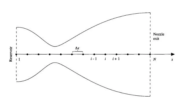
Note :- For the ease of programming we will drop the use of the prime to denote a dimensionless variable.

• For Non-conservation form

First we will do the predictor step , in which we will apply forward differencing on the spatial derivatives,

We get the governing equations as ,

Continuity equation,

`((delrho)/(delt))_i^(t)=-rho_i^(t)(V_(i+1)^(t)-V_i^(t))/(Deltax)-rho_i^(t)V_i^(t)(lnA_(i+1)-lnA_(i))/(Deltax)-V_i^(t)(rho_(i+1)^(t)-rho_i^(t))/(Deltax)`

Momentum equation,

`((delV)/(delt))_i^(t)=-V_i^(t)(V_(i+1)^(t)-V_i^(t))/(Deltax)-(1/gamma)((T_(i+1)^(t)-T_i^(t))/(Deltax)+T_i^(t)/rho_i^(t)(rho_(i+1)^(t)-rho_i^(t))/(Deltax))`

Energy equation,

`((delT)/(delt))_i^(t)=-V_i^(t)(T_(i+1)^(t)-T_i^(t))/(Deltax)-(gamma-1)T_i^(t)[(V_(i+1)^(t)-V_i^(t))/(Deltax)+V_i^(t)(lnA_(i+1)-lnA_(i))/(Deltax)]`

Here `t` is the initial time step at which the values of flow variables are known.

Now we will find the predicted values of the flow variables,

`rho_i^(t+Deltat)=rho_i^(t)+((delrho)/(delt))_i^(t)(Deltat)`

`V_i^(t+Deltat)=V_i^(t)+((delV)/(delt))_i^(t)(Deltat)`

`T_i^(t+Deltat)=T_i^(t)+((delT)/(delt))_i^(t)(Deltat)`

Here `Deltat` is the time step value.

Now let us do the corrector step, in this step we will apply rearward difference on the spatial derivatives,

Continuity equation,

`((delrho)/(delt))_i^(t+Deltat)=-rho_i^(t+Deltat)(V_(i)^(t+Deltat)-V_(i-1)^(t+Deltat))/(Deltax)-rho_i^(t+Deltat)V_i^(t+Deltat)(lnA_(i)-lnA_(i-1))/(Deltax)-V_i^(t+Deltat)(rho_(i)^(t+Deltat)-rho_(i-1)^(t+Deltat))/(Deltax)`

Momentum equation,

`((delV)/(delt))_i^(t+Deltat)=-V_i^(t+Deltat)(V_(i)^(t+Deltat)-V_(i-1)^(t+Deltat))/(Deltax)-(1/gamma)((T_(i)^(t+Deltat)-T_(i-1)^(t+Deltat))/(Deltax)+T_(i)^(t+Deltat)/rho_i^(t+Deltat)((rho_(i)^(t+Deltat)-rho_(i-1)^(t+Deltat))/(Deltax)))`

Energy equation,

`((delT)/(delt))_i^(t+Deltat)=-V_i^(t+Deltat)(T_(i)^(t+Deltat)-T_(i-1)^(t+Deltat))/(Deltax)-(gamma-1)T_i^(t+Deltat)[(V_(i)^(t+Deltat)-V_(i-1)^(t+Deltat))/(Deltax)+V_i^(t+Deltat)(lnA_(i)-lnA_(i-1))/(Deltax)]`

Now we will find the average time derivative values as shown below,

`((delrho)/(delt))_(av)=0.5[ubrace(((delrho)/(delt))_i^(t))_("predictor")+ubrace(((delrho)/(delt))_i^(t+Deltat))_("corrector")]`

`((delV)/(delt))_(av)=0.5[ubrace(((delV)/(delt))_i^(t))_("predictor")+ubrace(((delV)/(delt))_i^(t+Deltat))_("corrector")]`

`((delT)/(delt))_(av)=0.5[ubrace(((delT)/(delt))_i^(t))_("predictor")+ubrace(((delT)/(delt))_i^(t+Deltat))_("corrector")]`

Finally the corrected value of the flow field variables at time `t+Deltat` are,

`rho_i^(t+Deltat)=rho_i^(t)+((delrho)/(delt))_(av)(Deltat)`

`V_i^(t+Deltat)=V_i^(t)+((delV)/(delt))_(av)(Deltat)`

`T_i^(t+Deltat)=T_i^(t)+((delT)/(delt))_(av)(Deltat)`

• For Conservation form

Let us convert those quasi one-dimensional flow equations into generic form.

To do so we have to define the elements of solutions vector U , the flux vector F and the source term J as given below,

`U_1 = rho^'A^'`

`U_2 = rho^'A^'V^'`

`U_3 = rho^'(e^'/(gamma-1)+gamma/2V^('2))A^'`

`F_1 = rho^'A^'V^'`

`F_2 = rho^'V^('2)A^'+(1"/"gamma)p^'A^'`

`F_3 = rho^'(e^'/(gamma-1)+gamma/2V^('2))V^'A^'+rho^'A^'V^'`

`J_2 = (1/gamma)p^'(delA^')/(delx^')`

By decoding the above equations we get the values of the primitive variables,

`rho^'=U_1/A^'`

`V^' = U_2/U_1`

`e^'=C_vT/(C_vT_0)=T/T_0=T^' ( since , e^'=e/(e_0) , e = C_vT)`

`p^'=rho^'T^'`

So the generic form will be as follows,

`(delU_1)/(delt^')=-(delF_1)/(delx^')`

`(delU_2)/(delt^')=-(delF_2)/(delx^')+J_2`

`(delU_3)/(delt^')=-(delF_3)/(delx^')`

Note :- For the ease of programming we will drop the use of the prime to denote a dimensionless variable.

Now the equations for these flux terms and the source term in terms of solution vector is as follows,

`F_1 = U_1`

`F_2 = U_2^2/(U_1)+(gamma-1)/gamma(U_3-gamma/2U_2^2/(U_1))`

`F_3 = gamma((U_2U_3)/U_1)-(gamma(gamma-1))/2(U_2^3/(U_1^2))`

`J_2 = (gamma-1)/gamma(U_3-gamma/2U_2^2/(U_1))(del(lnA))/(delx)`

Now let us do the predictor step on these generic equations we have derived , in which we will apply forward differencing on the x derivatives,

`((delU_1)/(delt))_i^(t)=-[((F_1)_(i+1)-(F_1)_i)/(Deltax)]`

`((delU_2)/(delt))_i^(t)=-[((F_2)_(i+1)-(F_2)_i)/(Deltax)]+J_2`

`((delU_3)/(delt))_i^(t)=-[((F_3)_(i+1)-(F_3)_i)/(Deltax)]`

Next we will calculate the predicted values as,

`(U_1)_i^(t+Deltat)=(U_1)_i^(t)+((delU_1)/(delt))_i^(t)Deltat`

`(U_2)_i^(t+Deltat)=(U_2)_i^(t)+((delU_2)/(delt))_i^(t)Deltat`

`(U_3)_i^(t+Deltat)=(U_3)_i^(t)+((delU_3)/(delt))_i^(t)Deltat`

Using these predicted values of the solution vector we will find the predicted values of `rho` and `T`.

Now we will calculate the predicted flux by putting the predicted solution vector values in the equations for flux in terms of `U`.

After that we will calculate the corrector step , in which we will apply rearward differencing on the x derivatives,

`((delU_1)/(delt))_i^(t+Deltat)=-[((F_1)_(i)-(F_1)_(i-1))/(Deltax)]`

`((delU_2)/(delt))_i^(t+Deltat)=-[((F_2)_(i)-(F_2)_(i-1))/(Deltax)]+J_2`

`((delU_3)/(delt))_i^(t+Deltat)=-[((F_3)_(i)-(F_3)_(i-1))/(Deltax)]`

Now we will find the average time derivative values as shown below,

`((delU_1)/(delt))_(av)=1/2[ubrace(((delU_1)/(delt))_i^(t))_("predictor")+ubrace(((delU_1)/(delt))_i^(t+Deltat))_("corrector")]`

`((delU_2)/(delt))_(av)=1/2[ubrace(((delU_2)/(delt))_i^(t))_("predictor")+ubrace(((delU_2)/(delt))_i^(t+Deltat))_("corrector")]`

`((delU_3)/(delt))_(av)=1/2[ubrace(((delU_3)/(delt))_i^(t))_("predictor")+ubrace(((delU_3)/(delt))_i^(t+Deltat))_("corrector")]`

Finally the corrected value of the solution vectors are,

`(U_1)_i^(t+Deltat)=(U_1)_i^(t)+((delU_1)/(delt))_(av)Deltat`

`(U_2)_i^(t+Deltat)=(U_2)_i^(t)+((delU_2)/(delt))_(av)Deltat`

`(U_3)_i^(t+Deltat)=(U_3)_i^(t)+((delU_3)/(delt))_(av)Deltat`

From these corrected values we can find the corrected primitive variable values.

PROGRAM

In this program we have 2 functions and 1 main program. The 2 function program will solve the equations in non-conservation form and the conservation form. The main program will call these function programs and will compare the results of the two.

First of all let us look at the function program for non-conservation form,

• Non-conservation form

  function [m_nc , x , rho_nc , M_nc , t_nc , nt,p_nc,n,fig4,fig5 ] = non_conservation_form 
  
  % number of grid points and the step size defined
  n=31;
  x=linspace(0,3,n);
  dx=x(2)-x(1);
  
  % initial values of flow variables defined
  rho_nc = 1-0.3146*x;
  t_nc = 1-0.2314*x;     % here t is temperature
  v_nc = (0.1+1.09*x).*t_nc.^0.5;
  a = 1+2.2*(x-1.5).^2;
  
  %ratio of specific heats at standard condition
  gamma = 1.4;
  
  % Courant number
  c=0.5;
  % time step calculation
  dt=min(c*dx./(sqrt(t_nc)+v_nc));
  
  %number of time steps
  nt=1400;
  
  % figure window
  figure (4)
  hold on
  %%
  % time loop
  for k=1:nt
      
      % storing old values
      rho_old = rho_nc;
      t_old = t_nc;
      v_old = v_nc;
      
      % predictor step
      for j=2:n-1
          
          %simplifying the calculation
          dv_dx = (v_nc(j+1)-v_nc(j))/dx;
          dlog_a_dx = (log(a(j+1))-log(a(j)))/dx;
          drho_dx = (rho_nc(j+1)-rho_nc(j))/dx;
          dt_dx = (t_nc(j+1)-t_nc(j))/dx;
          
          % continuity equation
          drho_dt_p(j) = -rho_nc(j)*(dv_dx)-rho_nc(j)*v_nc(j)*(dlog_a_dx)-v_nc(j)*(drho_dx);
          
          % momentum equation
          dv_dt_p(j) = -v_nc(j)*(dv_dx)-(1/gamma)*(dt_dx+(t_nc(j)/rho_nc(j))*drho_dx);
          
          % energy equation 
          dt_dt_p(j) = -v_nc(j)*dt_dx-(gamma-1)*t_nc(j)*[dv_dx+v_nc(j)*(dlog_a_dx)];
          
          % predicted values
          rho_nc(j) = rho_nc(j) +  drho_dt_p(j)*dt;
          v_nc(j) = v_nc(j) +  dv_dt_p(j)*dt;
          t_nc(j) = t_nc(j) +  dt_dt_p(j)*dt;
          
      end
      
      % corrector step
        for j=2:n-1
            
          %simplifying the calculation
          dv_dx = (v_nc(j)-v_nc(j-1))/dx;
          dlog_a_dx = (log(a(j))-log(a(j-1)))/dx;
          drho_dx = (rho_nc(j)-rho_nc(j-1))/dx;
          dt_dx = (t_nc(j)-t_nc(j-1))/dx;
          
          % continuity equation
          drho_dt_c(j) = -rho_nc(j)*(dv_dx)-rho_nc(j)*v_nc(j)*(dlog_a_dx)-v_nc(j)*(drho_dx);
          
          % momentum equation
          dv_dt_c(j) = -v_nc(j)*(dv_dx)-(1/gamma)*(dt_dx+(t_nc(j)/rho_nc(j))*drho_dx);
          
          % energy equation 
          dt_dt_c(j) = -v_nc(j)*dt_dx-(gamma-1)*t_nc(j)*[dv_dx+v_nc(j)*(dlog_a_dx)];
          
       end
          
          % average time derivative values
          drho_dt = 0.5*[drho_dt_p + drho_dt_c];
          dv_dt = 0.5*[dv_dt_p +  dv_dt_c];
          dt_dt = 0.5*[dt_dt_p + dt_dt_c];
          
          % corrected values of the flow variables calculated
          for i=2:n-1
              
              rho_nc(i) = rho_old(i) +  drho_dt(i)*dt;
              v_nc(i) = v_old(i) +  dv_dt(i)*dt;
              t_nc(i) = t_old(i) +  dt_dt(i) *dt;
              
          end
          
          %boundary conditions
          %inlet
          v_nc(1) = 2*v_nc(2)-v_nc(3);
          
          %outlet
          v_nc(n) = 2*v_nc(n-1) - v_nc(n-2);
          rho_nc(n) = 2*rho_nc(n-1) - rho_nc(n-2);
          t_nc(n) = 2*t_nc(n-1) - t_nc(n-2);
  
          % storing the flow variable values 
          % at throat section for each time step
           rho_n(k)=rho_nc((n+1)/2);
           v_n(k) = v_nc((n+1)/2);
           t_n(k)=t_nc((n+1)/2);
          
        % to plot mass flow value at specified time step
        if k==50 || k==100  ||  k==150   ||  k==200   ||  k==1400   
            
            %calculating the mass flow at the specified time step
            m_nc = rho_nc.*v_nc.*a;
            %plotting mass flow rate vs length at different time step
            plot(x,m_nc,'LineWidth',3)
            
        end
    
  end
  %%
  
      lgd=legend('50','100','150','200','1400','location','best');
      lgd.Title.String = 'Number of time steps';
      title({sprintf('Non-conservation form (n=%d)',n);'Non-dimensional mass flow rate Vs Length at different time steps'},'FontWeight','bold','color','b','FontSize',18)
      xlabel('Nozzle length','FontWeight','bold','FontSize',13,'color','r')
      ylabel('Mass flow rate','FontWeight','bold','FontSize',13,'color','r')
      
       % Steady state pressure & mach number calculation at each grid point
       p_nc= rho_nc.*t_nc;
       M_nc =  v_nc./sqrt(t_nc);
       
      % calculating the pressure & mach number at throat section for each
      % time step     
       M_n = v_n./sqrt(t_n);
       p_n=rho_n.*t_n;
      
      % creating a array with size equal to number of time steps
      nts=(1:nt);
      
       % plotting flow variable characteristics for throat section at each
       % time step
      figure(5)
      subplot(4,1,1)
      plot(nts,rho_n,'LineWidth',3)
      title({sprintf('Non-conservation form (n=%d)',n);'Timewise variations of flow field variables at the nozzle throat'},'FontWeight','bold','color','b','FontSize',18)
      ylabel('Density','FontWeight','bold','color','r')
      subplot(4,1,2)
      plot(nts,M_n,'LineWidth',3)
      ylabel('Mach number','FontWeight','bold','color','r')
      subplot(4,1,3)
      plot(nts,t_n,'LineWidth',3)
      ylabel('Temperature','FontWeight','bold','color','r')
      subplot(4,1,4)
      plot(nts,p_n,'LineWidth',3)
      ylabel('Pressure','FontWeight','bold','color','r')
      xlabel('Number of time steps','FontWeight','bold','color','r','FontSize',13)
  
  % storing the figures as outputs    
  fig4 = figure(4);
  fig5 = figure(5);
  end
  

• The function output variables and the function name has been defined at the start of the programming.
• Then the number of grid points is specified , along with the step size.
• Then the initial conditions of the primitive variables has been defined. For this we have used the following equations,

`rho=1-0.3146x`

`T = 1-0.2314x`

`V = (0.1+1.09x)T^(1//2)`

`A = 1+2.2(x-1.5)^2`

Note :- For the ease of programming we have used small letters to denote velocity, temperature and area.

• Next we have defined the ratio of specific heats for air at standard condition.
• The Courant number used is `0.5` , as this value is less than unity we will get stable results.
• Then the time step value is selected such that it is the minimum of the `Deltat` value calculated as shown below,

`Deltat = C((Deltax)/(V+a))`

Where , `Deltax` is the step size , `V` is the velocity at each grid point and ‘a’ is the local speed of sound calculated as `a=sqrt(T)`.

• Number of time steps is specified.
• A figure window is called which is numbered as 4 and ‘hold on’ command is used to hold this figure window till the for loop for time step finishes. This step is necessary so as to plot graph showing variation with respect to number of time steps.
• Now the for loop is opened which runs for iterations equal to the number of time steps specified.
• To store the values of primitive variables calculated in the previous time step we have created three variables named with extension ‘old’.
• Now we will start calculating the intermediate numerical results. These calculations will not include initial and boundary values.
• Another for loop is opened which will run for iterations equal to (number of grid points - 1).
• Inside this for loop the the predictor step is calculated. Also for simplifying the code , the x derivatives has been defined separately , this will make the predictor step calculation much cleaner.
• The values of the primitive variables are the updated , which gives us the predicted values of those.
• For loop ended.
• Next for loop is opened , this used to calculate the corrector step.
• Inside this for loop we have calculated the corrector step by simplifying the equations as we have done for predictor step calculations.
• For loop ended.
• Then the average time derivative values are found out.
• Now to find the corrected values we have opened for loop , inside this we will calculate the corrected values of the primitive variables. For loop closed after that.
• Finally we will define the boundary conditions at inlet and the outlet.
• Here we have chosen velocity to be floating at the inflow and hence only it’s value has to be defined at the inlet. Other primitive variables are considered to be their respective stagnation values , i.e `rho_1 = 1` & `T_1 = 1`.
• Velocity at the inlet is given by ,

`V_1=2V_2-V_3`

• At the outlet we have to define all three flow variables. They are calculated by linear extrapolation as given below,

`V_n = 2V_(n-1)-V_(n-2)`

`rho_n = 2V_(n-1)-V_(n-2)`

`T_n = 2V_(n-1)-V_(n-2)`

Where ‘n’ is the number of grid points.

• To plot the flow variable characteristics at the throat section with respect to number of time steps , we have to store the values of flow variables at grid point `16` for each time steps.
• To plot the non-dimensional mass flow rate at specified time steps we have used if statement with ‘OR’ logical condition. Inside this if statement we will calculate the mass flow rate at that number of time step and will plot those. Formula for mass flow rate is , `dotm = rhoVA`
• The time loop is closed.
• Now the remaining graphs are plotted and these are stored as figures inside the function output.
• For plotting graphs showing variations of pressure and mach number we have calculated these using the formulas given below,

`P = rhoT`

`M = V/(sqrt(T))`

• Conservation form

  function [m_c , x, rho_c , M_c , t_c , nt,p_c,n,fig6,fig7 ] = conservation_form 
  
  % number of grid points and the step size defined
  n=31;
  x=linspace(0,3,n);
  dx=x(2)-x(1);
  
  % initial values of density and temperature calculated
  for i = 1:length(x)
      % here t is temperature array
  if x(i)>=0 && x(i)<0.5 
      rho_c(i)=1;
      t_c(i)=1;     
      
  else if x(i)>=0.5 && x(i)<=1.5
          rho_c(i)=1-0.366*(x(i)-0.5);
          t_c(i)=1-0.167*(x(i)-0.5);
          
      else if x(i)>1.5 && x(i)<=3.5
              rho_c(i) = 0.634 - 0.3879*(x(i) - 1.5) ;
              t_c(i) = 0.833 - 0.3507*(x(i) - 1.5);
          end
      end
  end
  end
  
  % initial values of area and velocity defined
  a = 1+2.2*(x-1.5).^2;
  v_c=0.59./(rho_c.*a);
  
  %ratio of specific heats at standard condition
  gamma = 1.4;
  
  %initial values of solution vector defined
  U1 = rho_c.*a;
  U2 = 0.59*ones(1,n);
  U3 = rho_c.*((t_c./(gamma-1))+(gamma.*v_c.^2)/2).*a;
  
  % Courant number
  c=0.5;
  % time step calculation
  dt=min(c*dx./(sqrt(t_c)+v_c));
  
  % number of time steps
  nt = 1400;
  
  %copy of initial temperature values
  t_old = t_c;
  
  % figure window
  figure (6)
  hold on
  %%
  % time loop
  for o=1:nt
      
       % storing old values
      U1_old = U1;
      U2_old = U2;
      U3_old = U3;
       
      % calculating initial flux terms
      F1 = U2;
      F2 =  (U2.^2./U1)+((gamma-1)/gamma)*(U3-((gamma*U2.^2)./(2*U1)));
      F3 = ((gamma*U2.*U3)./U1)-((gamma*(gamma-1))/2)*(U2.^3./U1.^2);
      
      % predictor step
  for k=1:n-1
          % initial source term value
      J2(k) = (rho_c(k)*t_c(k)*(a(k+1)-a(k)))/(gamma*dx);
      
       % forward differencing of x derivative
       dU1_dt(k) = (-F1(k+1)+F1(k))/dx;
       dU2_dt(k) = ((-F2(k+1)+F2(k))/dx)+J2(k);
       dU3_dt(k) = (-F3(k+1)+F3(k))/dx;
       
       % predicted values
       U1_p(k) = U1_old(k)+(dU1_dt(k)*dt);
       U2_p(k) = U2_old(k)+(dU2_dt(k)*dt);
       U3_p(k) = U3_old(k)+(dU3_dt(k)*dt);
       
       % predicted density and temperature values
       rho_p(k) =  U1_p(k)/a(k);
       t_p(k) = (gamma-1)*((U3_p(k)/U1_p(k))-(gamma/2)*(U2_p(k)/U1_p(k))^2);
       
  end
  
      % predicted flux values
      F1_p = U2_p;
      
      F2_p = (U2_p.^2./U1_p)+((gamma-1)/gamma)*(U3_p-((gamma*U2_p.^2)./(2*U1_p)));
  
      F3_p = ((gamma*U2_p.*U3_p)./U1_p)-((gamma*(gamma-1))/2)*(U2_p.^3./U1_p.^2);
      
  
  for m=2:n-1
      
        % corrector step
       dU1_dt_c(m) = (-F1_p(m)+F1_p(m-1))/dx;
       
       dU2_dt_c(m) = ((-F2_p(m)+F2_p(m-1))/dx)+((rho_p(m)*t_p(m)*(a(m)-a(m-1)))/(gamma*dx));
       
       dU3_dt_c(m) = (-F3_p(m)+F3_p(m-1))/dx;
       
  end
  
       % average time derivative value
       dU1_dt_av = 0.5*(dU1_dt+dU1_dt_c);
       dU2_dt_av = 0.5*(dU2_dt+dU2_dt_c);
       dU3_dt_av = 0.5*(dU3_dt+dU3_dt_c);
       
       for y=2:n-1
           
           % corrected values
           U1(y) = U1_old(y)+dU1_dt_av(y)*dt;
           U2(y) = U2_old(y)+dU2_dt_av(y)*dt;
           U3(y) = U3_old(y)+dU3_dt_av(y)*dt;
           
       end
           
       % corrected flow variable values
           rho_c =  U1./a;
           v_c = U2./U1;
           t_c = (gamma-1)*((U3./U1)-(gamma/2)*(v_c).^2);
       
       %boundary conditions
       % inlet values
       U1(1) = a(1);
       U2(1) = 2*U2(2)-U2(3);
       U3(1) = U1(1)*((t_old(1)/(gamma-1))+(gamma/2)*v_c(1).^2);
       
       % outlet values
       U1(n) = 2*U1(n-1)-U1(n-2);
       U2(n) = 2*U2(n-1)-U2(n-2);
       U3(n) = 2*U3(n-1)-U3(n-2);
  
        % storing the flow variable values 
        % at throat section for each time step
       rho_n(o)=rho_c((n+1)/2);
        v_n(o) = v_c((n+1)/2);
        t_n(o)=t_c((n+1)/2);
        
        % to plot mass flow value at specified time step
        if o==50 || o==100  ||  o==150   ||  o==200   ||  o==1400   
            %calculating the mass flow at the specified time step
            m_c = rho_c.*v_c.*a;
            %plotting mass flow rate vs length at different time step
            plot(x,m_c,'LineWidth',3)
            
        end
        
  end
   %%
  
      lgd=legend('50','100','150','200','1400','location','best');
      lgd.Title.String = 'Number of time steps';
      title({sprintf('Conservation form (n=%d)',n);'Non-dimensional mass flow rate Vs Length at different time steps'},'FontWeight','bold','color','b','FontSize',18)
      xlabel('Nozzle length','FontWeight','bold','FontSize',13,'color','r')
      ylabel('Mass flow rate','FontWeight','bold','FontSize',13,'color','r')
      
       % Steady state pressure & mach number calculation at each grid point
       p_c= rho_c.*t_c;
       M_c =  v_c./sqrt(t_c);
       
       % calculating the pressure & mach number at throat section for each
       % time step     
       p_n=rho_n.*t_n;
       M_n = v_n./sqrt(t_n);
       
       % creating a array with size equal to number of time steps
       nts=(1:nt);
  
      % plotting flow variable characteristics for throat section at each
      % time step
      figure(7)
      subplot(4,1,1)
      plot(nts,rho_n,'LineWidth',3)
      title({sprintf('Conservation form (n=%d)',n);'Timewise variations of flow field variables at the nozzle throat'},'FontWeight','bold','color','b','FontSize',18)
      ylabel('Density','FontWeight','bold','color','r')
      subplot(4,1,2)
      plot(nts,M_n,'LineWidth',3)
      ylabel('Mach number','FontWeight','bold','color','r')
      subplot(4,1,3)
      plot(nts,t_n,'LineWidth',3)
      ylabel('Temperature','FontWeight','bold','color','r')
      subplot(4,1,4)
      plot(nts,p_n,'LineWidth',3)
      ylabel('Pressure','FontWeight','bold','color','r')
      xlabel('Number of time steps','FontWeight','bold','color','r','FontSize',13)
  
  % storing the figures as outputs      
  fig6 = figure(6);
  fig7 = figure(7);
  end
  
  

• The function output variables and the function name has been defined at the start of the programming.
• Then the number of grid points is specified , along with the step size.
• Then the initial conditions of the primitive variables has been defined. For this we have used the following equations,

`{:(rho = 1),(T = 1):}}"for " 0<=x<=0.5`

`{:(rho=1-0.366(x-0.5)),(T=1-0.167(x-0.5)):}}"for " 0.5<=x<=1.5`

`{:(rho = 0.634 - 0.3879(x- 1.5)),( T = 0.833 - 0.3507(x- 1.5)):}}"for " 1.5<=x<=3.5`

`A = 1+2.2(x-1.5)^2`

`V = U_2/(rhoA)` , here `U_2` is taken as constant `0.59`

Note :- For the ease of programming we have used small letters to denote velocity, temperature and area.

• Next we have defined the ratio of specific heats for air at standard condition.
• Initial conditions for solution vectors , `U_1` , `U_2` & `U_3` are calculated using the derived formulas. Here we have taken `U_2` to be constant value of `0.59` since this solution vector represents the local mass flow and the exact analytical value of steady state mass flow is `0.579`.
• The Courant number used is `0.5` , as this value is less than unity we will get stable results.
• Then the time step value is selected such that it is the minimum of the Deltat value calculated as shown below,

`Deltat = C((Deltax)/(V+a))`

Where , `Deltax` is the step size , `V` is the velocity at each grid point and ‘a’ is the local speed of sound calculated as `a=sqrt(T)`.

• Number of time steps is specified.
• A copy of the initial value of temperature is stored as it is needed for calculations.
• A figure window is called which is numbered as 6 and ‘hold on’ command is used to hold this figure window till the for loop for time step finishes. This step is necessary so as to plot graph showing variation with respect to number of time steps.
• Now the for loop is opened which runs for iterations equal to the number of time steps specified.
• To store the values of solution vectors calculated in the previous time step we have created three variables named with extension ‘old’.
• After that we have calculated the flux term values using solution vectors.
• Now we will start calculating the intermediate numerical results. These calculations will not include initial and boundary values.
• So for that we have opened a for loop which runs for iterations equal to (number of grid points -1).
• Inside this for loop we will calculate the source term value and the predictor step. Also the predicted values of the solution vector and the flow variables are calculated inside this for loop.
• For loop is closed.
• Using the predicted values of the solution vector we will calculate the predicted values of flux terms.
• Another for loop is opened , inside which we will calculate the corrector step. For loop closed after that.
• Then the average time derivative values are found out.
• Now to find the corrected values we have opened a for loop , inside this we will calculate the corrected values of the solution vector. For loop closed after that.
• Using the corrected values of the solution vector we will calculate the flow variables value.
• Finally we will define the boundary conditions at inlet and the outlet.
• At inlet the values of the solution vector is calculated as follows,

`(U_1)_(i=1) = (rhoA)_(i=1)` , here `rho` is fixed and its value is `1`.

`(U_2)_(i=1) = (2U_2)_(i=2)-(U_2)_(i=3)`

`(U_3)_(i=1) = (U_1)_(i=1)(T/(gamma-1)+gamma/2V_(i=1)^(2))` , here `T` is fixed and its value is `1`.

• At outlet the values of the solution vector is calculated by linear extrapolation as follows,

`(U_1)_n = 2(U_1)_(n-1)-(U_1)_(n-2)`

`(U_2)_n = 2(U_2)_(n-1)-(U_2)_(n-2)`

`(U_3)_n = 2(U_3)_(n-1)-(U_3)_(n-2)`

Where ‘n’ is the number of grid points.

• To plot the flow variable characteristics at the throat section with respect to number of time steps , we have to store the values of flow variables at grid point `16` for each time steps.
• To plot the non-dimensional mass flow rate at specified time steps we have used if statement with ‘OR’ logical condition. Inside this if statement we will calculate the mass flow rate at that number of time step and will plot those.Formula for mass flow rate is , `dotm = rhoVA`
• The time loop is closed.
• Now the remaining graphs are plotted and these are stored as figures inside the function output.
• For plotting graphs showing variations of pressure and mach number we have calculated these using the formulas given below,

`P = rhoT`

`M = V/(sqrt(T))`

• Main program

  clear all
  close all
  clc
  
  % calling conservation form function program
  [m_c , x, rho_c , M_c , t_c , nt,p_c,n,fig6,fig7 ] = conservation_form ;
  % calling non-conservation form function program
  [m_nc , x , rho_nc , M_nc , t_nc , nt,p_nc,n,fig4,fig5  ] = non_conservation_form ;
  
  % plotting the comparison between the two forms
  figure(1)
  plot(x,m_c,'LineWidth',3)
  hold on
  plot(x,m_nc,'LineWidth',3)
  legend('Conservation form ','Non-conservation form','location','best')
  title(sprintf('Comparison of the steady-state mass flow variations (n=%d)',n) ,'FontWeight','bold','color','b','FontSize',18)
  ylabel('Non-dimensional mass flow rate','FontWeight','bold','color','r','FontSize',13)
  xlabel('Nozzle length','FontWeight','bold','color','r','FontSize',13)
  
  
          %plotting variation of flow variables at steady state for
          %non-conservation form
          figure(2)
          plot(x,M_nc,'LineWidth',3)
          hold on
          plot(x,rho_nc,'LineWidth',3)
          hold on
          plot(x,t_nc,'LineWidth',3)
          hold on
          plot(x,p_nc,'LineWidth',3)
          legend('Mach number','Density','Temperature','Pressure','location','best')
          title({sprintf('Non-conservation form (n=%d)',n);'Variation of flow variables in the nozzle at steady state'},'FontWeight','bold','color','b','FontSize',18)
          xlabel('Nozzle length','FontWeight','bold','color','r','FontSize',13)
          ylabel('Non-dimensional flow variable values','FontWeight','bold','color','r','FontSize',13)
          
          %plotting variation of flow variables at steady state for
          %conservation form       
          figure(3)
          plot(x,M_c,'LineWidth',3)
          hold on
          plot(x,rho_c,'LineWidth',3)
          hold on
          plot(x,t_c,'LineWidth',3)
          hold on
          plot(x,p_c,'LineWidth',3)
          legend('Mach number','Density','Temperature','Pressure','location','best')
          title({sprintf('Conservation form (n=%d)',n);'Variation of flow variables in the nozzle at steady state'},'FontWeight','bold','color','b','FontSize',18)
          xlabel('Nozzle length','FontWeight','bold','color','r','FontSize',13)
          ylabel('Non-dimensional flow variable values','FontWeight','bold','color','r','FontSize',13)
  

• In this program we will call the function programs that we have written already.
• After calling those function programs we will plot a graph comparing the non-dimensional mass flow rate value calculated by non-conservation form and the conservation form.
• From this plot we can understand the difference between the two forms of equations.
• Also graphs showing the variation of flow variables at steady state with respect to length is plotted for both the forms.

RESULTS

The results when the number of grid point is 31 is given below.

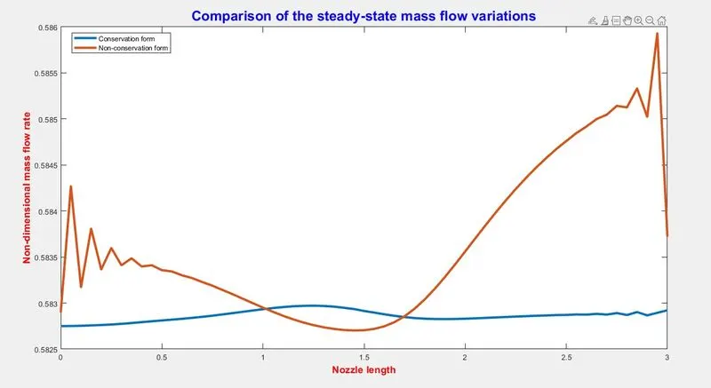
Comparison of conservation form with non-conservation form

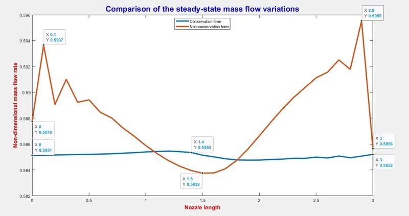
From this plot we can understand that the conservation form gives almost constant result.

Whereas the non-conservation form gives us variable result , i.e the result is not constant along the length of the nozzle. We can see that at the inlet and the outlet there is a spike in the values.

So we can conclude that the conservation form gives us flux values that are much closer to the analytical values and are also constant throughout the length of the nozzle. This happened because in the conservation form the mass flow rate itself is one of the dependent variable in the equations but in case of non-conservation form it is obtained as a secondary result. Hence the conservation form conserves the mass throughout the flow field better than non-conservation form.

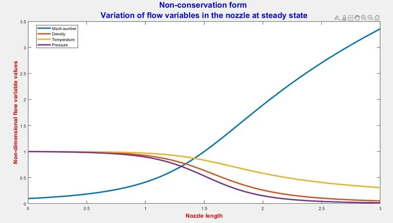
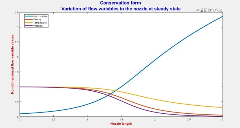
Variation of flow variables in the nozzle at steady state

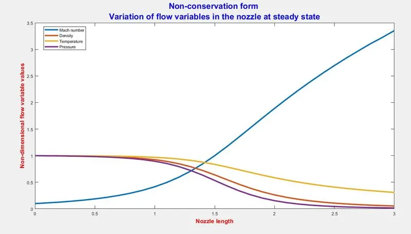
• Non-conservation form

• Conservation form

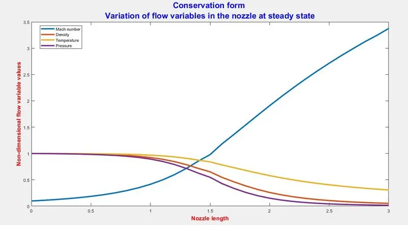
On comparing these two graphs we can understand that the values of flow variables calculated using non-conservation form and conservation form are almost the same. When these values are compared to the actual analytical values we can find that the non-conservation form values are much closer to the analytical values.

So we can conclude that the non-conservation form leads to slightly more accurate results for primitive variables.

Time wise variations of flow field variables at the nozzle throat

• Non-conservation form

• Conservation form

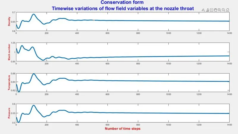
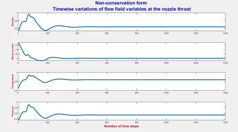
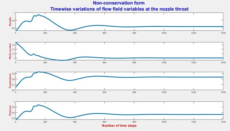
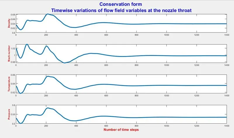
By comparing these two plots we can find that the flow variables change rapidly in case of conservation compared to non-conservation form. This effect of rapid change at the earlier stages is called rubber band effect . This effect is high in case of conservation form.

Also the time taken to reach steady state is comparatively high for conservation form.

Variation of non-dimensional mass flow rate along the nozzle at different time step

• Non-conservation form

• Conservation form

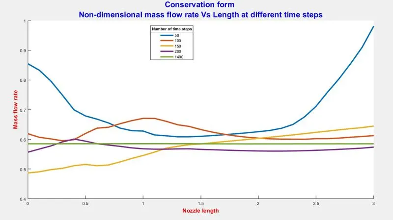
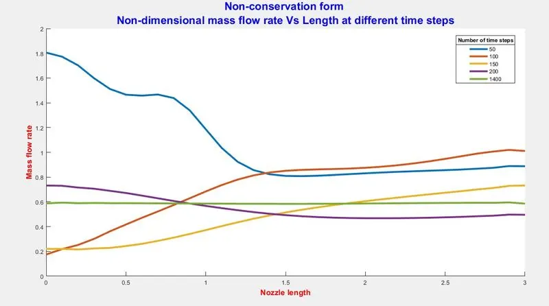
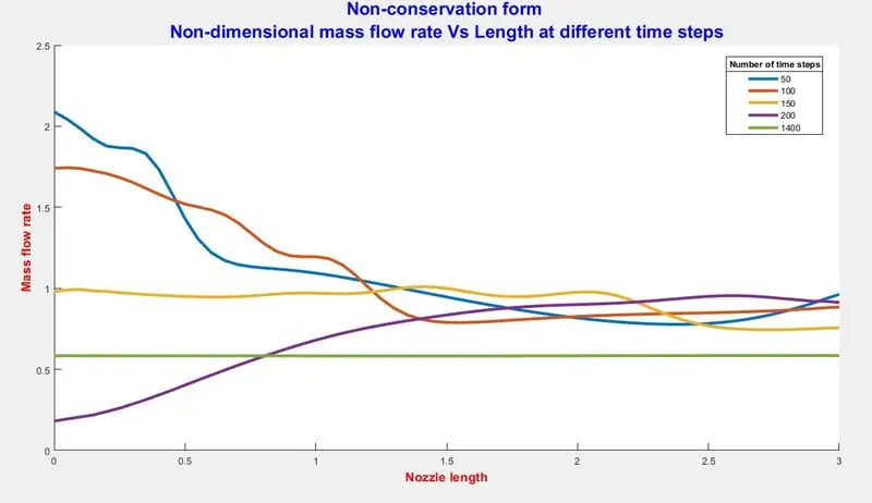
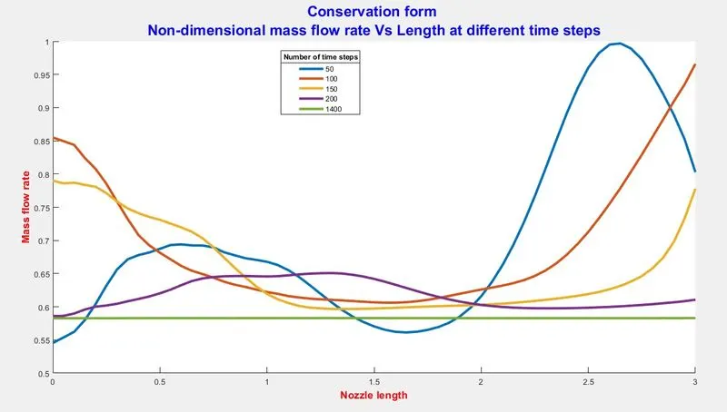
Here we can see that in both the graphs after 200 time steps the mass flow distribution starts to settle down. But the difference is that in conservation form the mass flow variations is much less at higher number of time steps and at the outlet the mass flow rate is very close to each other at different time steps.

At 50 number of time steps we can see that non-conservation form is decreasing where as the conservation form decreases and then rapidly increases , so we can say that at lower number of time steps non-conservation form has more constant characteristics.

At 1400 number of time steps both the forms attains steady state. The only difference being that the steady state value of conservation form is much closer to actual analytical solution.

Grid independence test

A grid independence test is a condition in which the number of grid points will no longer affect the solution values. To achieve grid independence we have to increase the number of grid points till our solution is no longer sensitive to the increase in number of grid points.

In our case we will test for grid independence by changing the number of grid points to 61.

Now let us run the program and check the results shown below,

Comparison of conservation form with non-conservation form

Variation of flow variables in the nozzle at steady state

• Non-conservation form

• Conservation form

Time wise variations of flow field variables at the nozzle throat

• Non-conservation form

• Conservation form

Variation of non-dimensional mass flow rate along the nozzle at different time step

• Non-conservation form

• Conservation form

Comparing these results with grid points equal to 31 , we get the following values,

Flow field variable values at `n^(th)` grid point (Steady state)
Form	`M`	`rho`	`T`	`p`
Conservation form (31 grid points)	3.376	0.05271	0.3055	0.0161
Conservation form (61 grid points)	3.363	0.05256	0.3072	0.01615
Non-conservation form (31 grid points)	3.353	0.05287	0.3083	0.0163
Non-conservation form (61 grid points)	3.358	0.05265	0.3079	0.01621

From this table we can understand that the values of flow field variables are almost the same at the two different number of grid points and hence we can say that our calculation is independent of number of grid points.

CONCLUSION

Simulation of the isentropic flow through a quasi 1-D subsonic-supersonic nozzle using both the conservation form and non-conservation form of governing equations has been done successfully and the graphs has been plotted and studied.