Week 12 - Validation studies of Symmetry BC vs Wedge BC in OpenFOAM vs Analytical H.P equation
AIM
To simulate an axi-symmetric flow by applying the wedge boundary condition and symmetry boundary condition using OpenFOAM software. Also highlight the differences in both boundary conditions in terms of their usage and application.
The wedge angles at which simulation has to be done are 10°,25° & 45°.
Also validate the results with the Hagen- Poiseuille's equations for the fully developed flow.
THEORY
The physics of the fluid inside a pipe is such that its velocity changes from zero at the surface to a maximum at the pipe center. Hence we uses average velocity for calculations as it remains constant in incompressible flow when the cross-sectional area of the pipe is constant.
Wedge boundary condition is used for 2-dimensional axi-symmetric cases. These axi-symmetric wedge planes must be specified as separate patches of wedge type.
Symmetry boundary condition is used for any patch which uses the symmetry plane condition. These are used to replicate the simulated results for the entire geometry , if that geometry is symmetrical. This boundary condition helps in reducing the the size of the geometry and making the computation faster.
GOVERNING EQUATIONS
The governing equations for a fully developed laminar flow are given below ,
The hydrodynamic entry length , `L_h ~= 0.05*Re*D`
Where Re is the Reynolds number and D is the diameter of the pipe.
Average velocity of the flow , `V_(avg) = (nu*Re)/D`
Where nu is the kinematic viscosity (`nu = mu/rho`)
Maximum velocity , `u_(max) = 2*V_(avg)`
Maximum shear stress , `tau_(max) = (2*mu*u_(max))/R`
Where `mu` is the dynamic viscosity and R is the radius of the pipe.
Pressure drop , `DeltaP = (32*mu*L*V_(avg))/D^2`
Where L is the distance between the two pressures measured at point 1 and point 2 as shown in the diagram given below,
OBJECTIVE
- To write a code in MATLAB to automate the generation of blockMeshDict file.
- To validate Hydro-dynamic length with the numerical result.
- To validate the fully developed flow velocity profile with its analytical profile.
- To validate maximum velocity and pressure drop for fully developed flow.
- To post-process shear stress and validate wall shear stress for fully developed flow.
ASSUMPTIONS
Diameter of the pipe is assumed to be `10mm` and the fluid to be water at `25^circ C`. The density of the water at this temperature is `997 (Kg)/m^3` , dynamic viscosity is `8.891"*"10^-4 (Kg)/(ms)` and kinematic viscosity is `8.917"*"10^-7 m^2/s`.
PROCEDURE
- Using the MATLAB script file we will create the required blockMeshDict file for different wedge angles. Then this file is copied to the OpenFOAM folder.
- The program is given below,
clear all close all clc % input values d= input('enter the diameter of the pipe : '); Re = input('enter the Reynolds number : '); theta=input('enter the wedge angle : '); nu = input('enter the kinematic viscosity of the fluid : '); rho = input('enter the density of the fluid : '); % total length of the pipe = hydrodynamic length + fully developed region l = (0.06*Re*d)+340; % radius of the pipe r=d/2; % selecting the type of boundary condition bc = input('\n enter 1 for wedge / enter 2 for symmetry : '); %% creating the blockMeshDict file f1=fopen('blockMeshDict.txt','w'); % unit=input('enter conversion to meter value : ') fprintf(f1,'FoamFile\n{\nversion 2.0;\nformat ascii;\nclass dictionary;\nobject blockMeshDict;\n}\n\n'); fprintf(f1,'convertToMeters %f;\n\n',0.001); % vertices fprintf(f1,'vertices\n(\n'); fprintf(f1,' (%f %f %f)\n', 0,0,0) ; fprintf(f1,' (%f %f %f)\n', l,0,0) ; fprintf(f1,' (%f %f %f)\n', l, r*cosd(theta/2),-r*sind(theta/2)) ; fprintf(f1,' (%f %f %f)\n', 0, r*cosd(theta/2),-r*sind(theta/2)); fprintf(f1,' (%f %f %f)\n', l, r*cosd(theta/2),r*sind(theta/2)) ; fprintf(f1,' (%f %f %f)\n', 0, r*cosd(theta/2),r*sind(theta/2)); fprintf(f1,');\n\n'); % blocks fprintf(f1,'blocks\n(\n'); fprintf(f1,' hex (%g %g %g %g %g %g %g %g)', 0 ,1,2,3,0,1,4,5); fprintf(f1,' (%g %g %g) simpleGrading (1 0.2 1)\n);\n\n', 300 , 50 ,1); % edges fprintf(f1,'edges\n(\n'); fprintf(f1,' arc 3 5 (0 %f 0)\n',r); fprintf(f1,' arc 2 4 (%f %f 0)\n',l,r); fprintf(f1,');\n\n'); % boundary fprintf(f1,'boundary\n(\n inlet\n {\n type patch;\n faces\n (\n (3 0 0 5)\n );\n }\n\n'); fprintf(f1,' outlet\n {\n type patch;\n faces\n (\n (2 4 1 1)\n );\n }\n\n'); % printing the boundary condition as per the input value if bc==1 fprintf(f1,' front\n {\n type wedge;\n faces\n (\n (5 0 1 4)\n );\n }\n\n'); fprintf(f1,' back\n {\n type wedge;\n faces\n (\n (3 2 1 0)\n );\n }\n\n'); else fprintf(f1,' front\n {\n type symmetry;\n faces\n (\n (5 0 1 4)\n );\n }\n\n'); fprintf(f1,' back\n {\n type symmetry;\n faces\n (\n (3 2 1 0)\n );\n }\n\n'); end fprintf(f1,' top\n {\n type wall;\n faces\n (\n (2 3 5 4)\n );\n }\n\n'); fprintf(f1,' bottom\n {\n type empty;\n faces\n (\n (0 1 1 0)\n );\n }\n'); fprintf(f1,');\n\n'); fclose(f1); %% %input value of section between which pressure drop is measured L = input('\n enter length of the pipe section (pressure drop) : ' ); % Analytical values for validating the simulated results fprintf('\n\n Analytical values\n') % Inlet velocity calculation v_avg = (nu*Re)/(d*10^-3); u_max = 2*v_avg; fprintf(' The average velocity is %f m/s \n',v_avg) fprintf(' The maximum velocity is %f m/s \n',u_max) % maximum stress tau_max = (2*nu*rho*u_max)/(r*10^-3); fprintf(' The maximum shear stress is %f N/m^2',tau_max) % Pressure drop delta_P = (32*L*rho*nu*v_avg)/(d*10^-3)^2; fprintf(' \n The pressure drop is %f N/m^2 \n',delta_P) %Hydrodynamic length L_h = (0.06*Re*d*10^-3); fprintf(' The Hydrodynamic length is %f m \n',L_h)
Wedge boundary condition
- In this case we will specify the boundary type as wedge for front and back face of the wedge geometry. This has to be specified in three files namely ‘blockMeshDict’ , initial condition for pressure file ‘p’ and initial condition for velocity file ‘U’.
- The average velocity value is taken as the inlet velocity and gauge pressure (at 1 atm) is taken as outlet pressure.
- Now we will create the block mesh using the ‘blockMesh’ command and then solved using the solver ‘icoFoam’ which isthe transient solver for incompressible, laminar flow of Newtonian fluids.
- After solving we will open the post-processor , paraview using the command ‘paraFoam’.
- Here we will run the simulation and plot the necessary graphs.
- To plot the shear stress we have to first calculate the magnitude of velocity U , and then find the gradient of this velocity. After that this gradient value has to be multiplied with dynamic viscosity of the fluid which gives us the shear stress value. All these calculations are done using built-in calculator of paraview and the gradient is found using Gradient of unstructured dataset tool.
Symmetry boundary condition
- In this case we will specify the boundary type as symmetry for front and back face of the wedge geometry. This has to be specified in three files namely ‘blockMeshDict’ , initial condition for pressure file ‘p’ and initial condition for velocity file ‘U’.
All other procedures are similar to that of wedge boundary condition till the post-processing of the shear stress.
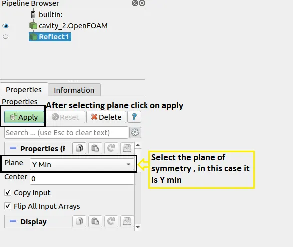
- In symmetry condition we can get the simulation results for the entire cross-section of the pipe. To get those results we have to use ‘Reflect’ tool. This tool will copy the results for the mirror image of the geometry along the symmetry plane. This is shown below,
RESULTS
Wedge boundary condition
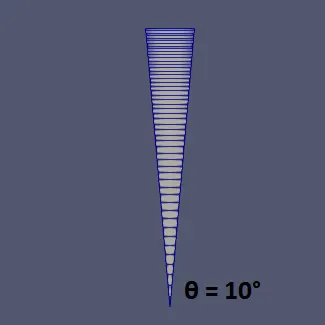
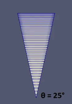
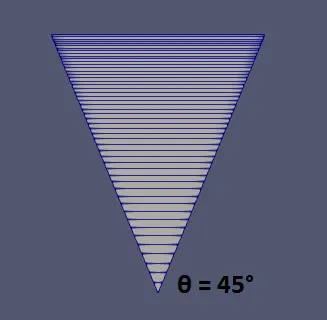
The geometry at wedge angles of 10°,25° and 45° are shown below,
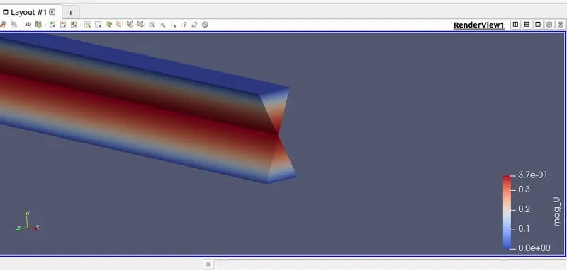
The simulation results are shown below,
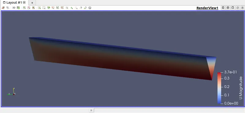
Symmetry boundary condition
The geometry at wedge angles of 10°,25° and 45° are shown below,
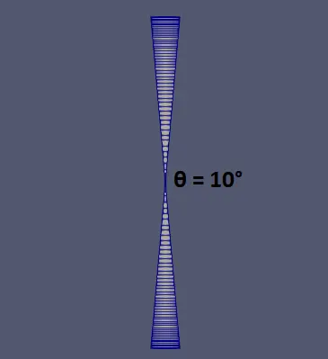
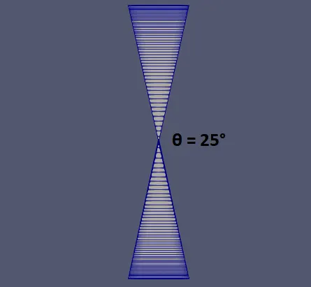
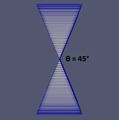
The simulation results are shown below,
Comparing the results of the two boundary conditions
From the plots we get the values of maximum velocity , hydrodynamic length , pressure drop and maximum shear stress.
We have to convert the pressure value that we get from the plot , which is kinematic pressure to dynamic pressure. This is done by multiplying density with kinematic pressure.
We have measured pressure drop for section between 1.3m and 1.6m of the pipe.
`"Dynamic pressure" = "Density" (rho) "* Kinematic pressure"`
Now we will compare these values to the analytical values got from the Hagen- Poiseuille's equations solved using the MATLAB codes in the below table for wedge angles `10°,25° & 45°` ,
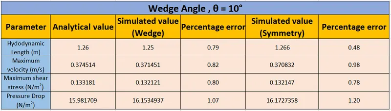
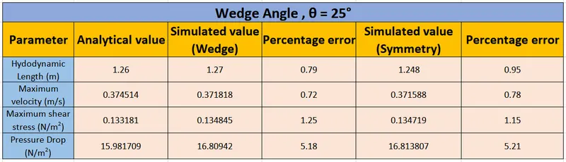
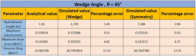
From these results we can find that as the wedge angle increases the error also increases. This has affected the pressure drop value severely as its error percentage increased from `1.2%` at `10°` to `17.3%` at `45°` for both wedge and symmetry boundary conditions.
On comparing wedge boundary condition and symmetry boundary condition we can see that the error percentage is less for wedge boundary condition for all flow parameters except shear stress.
But this difference is not that significant and hence we can use both of them as per our requirement and get accurate results.
CONCLUSION
An axi-symmetric flow by applying the wedge boundary condition and symmetry boundary condition using OpenFOAM software has been simulated successfully and the results has been validated using Hagen- Poiseuille's equations for the given set of wedge angles. Also a comparison between wedge boundary condition and symmetry boundary condition has been done.