Week 5.1 - Mid term project - Solving the steady and unsteady 2D heat conduction problem

AIM

To perform the Steady state analysis & Transient State analysis on 2D heat conduction equation by using the point iterative techniques.

The Boundary conditions for the problem are as follows;

Top Boundary = 600 K

Bottom Boundary = 900 K

Left Boundary = 400 K

Right Boundary = 800 K

THEORY

Steady state is the condition in which the temperature or the heat flux remains unchanged with time at any point within the medium.

Equation for steady state is ,

`(delta^2T)/(deltax^2) + (delta^2T)/(deltay^2) = 0` ---Eq(1)

Transient state is the condition in which the temperature or the heat flux varies with time and hence they are time dependent.

Equation of 2D transient heat conduction is,

`(deltaT)/(deltat) = alpha((delta^2T)/(deltax^2) + (delta^2T)/(deltay^2))` ---Eq(2)

Where alpha is the thermal diffusivity.

For solving implicit equations we use iterative methods. These methods are based on the repeated application of a relatively simple algorithm leading to eventual convergence. Examples of such methods are Jacobi , Gauss-Seidel & Successive Over Relaxation method (SOR).

The Jacobi and Gauss–Seidel methods are general-purpose point-iterative algorithms that are easily implementable, but their convergence rate can be slow when the system of equations is large, where as the SOR method is an extension of these two methods so as to eliminate that drawback and has a faster convergence rate comparatively.

OBJECTIVE

To solve the equations using the point iterative techniques Jacobi , Gauss-Seidel and Successive Over Relaxation (SOR) with absolute error value criteria at 1e-4.

DERIVATION

• For steady state

Applying central differencing on equation(1) we get ,

`(T_R-2T_P+T_L)/(Deltax^2) + (T_T-2T_P+T_B)/(Deltay^2)` = 0

Rearranging this we get ,

`T_P = (Deltay^2)/(2(Deltax^2+Deltay^2))(T_R+T_L)+(Deltax^2)/(2(Deltax^2+Deltay^2))(T_T+T_B)`

Now multiplying and dividing `Deltax^2` on the first part of RHS & `Deltay^2` on the second part of RHS , we get,

`T_P = (Deltay^2*Deltax^2)/(2(Deltax^2+Deltay^2))((T_R+T_L)/(Deltax^2))+(Deltay^2*Deltax^2)/(2(Deltax^2+Deltay^2))((T_T+T_B)/(Deltay^2))`

Let , `K = (2(Deltax^2+Deltay^2))/(Deltay^2*Deltax^2)`

`T_P = 1/K((T_R+T_L)/(Deltax^2))+1/K((T_T+T_B)/(Deltay^2))` ---Eq(3)

Where , `T_P = T_(i,j)` , `T_R = T_(i+1,j)` , `T_L=T_(i-1,j)` , `T_T=T_(i,j+1)` , `T_B=T_(i,j-1)`

For getting solution using Jacobi method use `T^"old"` on all terms in R.H.S of the equation (3). Where `T^"old"` represents the value of that node in the previous position. The equation will be as follows,

`T_(i,j)= 1/K((T_(i+1,j)^"old"+T_(i-1,j)^"old")/(Deltax^2))+1/K((T_(i,j+1)^"old"+T_(i,j-1)^"old")/(Deltay^2))`

For getting solution using Gauss-Seidel use `T^"old"` only for the terms that will be calculated after `T_(i,j)` in the R.H.S of the equation (3), this means that the value of those nodes that is already calculated in the current position are used to calculate nodes coming after in the same position. The equation will be as follows,

`T_(i,j)= 1/K((T_(i+1,j)^"old"+T_(i-1,j))/(Deltax^2))+1/K((T_(i,j+1)^"old"+T_(i,j-1))/(Deltay^2))` ---Eq(4)

Now for SOR method , it is an extension of Gauss-Seidel method and hence the equation is like,

`T_(i,j)= (1-omega)T_(i,j)^"old" + omega[ T_(GS) ]`

Where , `T_(GS)` is the equation for Gauss-Seidel , i.e equation(4) and `omega` is the relaxation factor.

• For transient state,

Applying forward differencing on the L.H.S and central differencing on the R.H.S on equation(2) , we get,

`(T_(i,j)^(n+1)-T_(i,j)^n)/(Deltat) = alpha[((T_(i+1,j)-2T_(i,j)+T_(i-1,j))/(Deltax^2))+((T_(i,j+1)-2T_(i,j)+T_(i,j-1))/(Deltay^2))]^n`

Rearranging this equation we get,

`T_(i,j)^(n+1) = T_(i,j)^n + alphaDeltat[((T_(i+1,j)-2T_(i,j)+T_(i-1,j))/(Deltax^2))+((T_(i,j+1)-2T_(i,j)+T_(i,j-1))/(Deltay^2))]^n` ---Eq(5)

Let `K_1 = (alphaDeltat)/(Deltax^2)` & `K_2 = (alphaDeltat)/(Deltay^2)`

Now putting this in equation (5) and simplyfying we get,

`T_(i,j)^(n+1) = [T_(i,j)^n + K_1(T_(i+1,j)^n+T_(i-1,j)^n)+K_2(T_(i,j+1)^n+T_(i,j-1)^n)]/(1+2K_1+2K_2)` ---Eq(6)

This is the equation for explicit solver.

Now let us derive the Implicit solver for transient state,

For this we have to replace ‘n’ with ‘n+1’ in equation (6) ,

`T_(i,j)^(n+1) = [T_(i,j)^(n(prev)) + K_1(T_(i+1,j)^(n+1)+T_(i-1,j)^(n+1))+K_2(T_(i,j+1)^(n+1)+T_(i,j-1)^(n+1))]/(1+2K_1+2K_2)` ---Eq(7)

This is the jacobi method.

For Gauss-Seidel method , we have to replace the terms in equation (7) that are already updated before calculating `T_(i,j)^(n+1)` , then the equation becomes,

`T_(i,j)^(n+1) = [T_(i,j)^(n(prev)) + K_1(T_(i+1,j)^(n+1)+T_(i-1,j)^n)+K_2(T_(i,j+1)^(n+1)+T_(i,j-1)^n)]/(1+2K_1+2K_2)` --Eq(8)

This is the required equation for Gauss-Seidel method.

NOTE : `T_(i,j)^(n(prev))` term on the R.H.S of equation (7) and equation (8) is the value of `T_(i,j)` in the previous time step.

Now for SOR method , as we have already explained , we have to just substitute equation (8) in equation given below,

`T_(i,j)^(n+1)= (1-omega)T_(i,j)^n + omega[ T_(GS) ]`

Here T_(GS) is the equation (8).

We get,

`T_(i,j)^(n+1)= (1-omega)T_(i,j)^n + omega[[T_(i,j)^(n(prev)) + K_1(T_(i+1,j)^(n+1)+T_(i-1,j)^n)+K_2(T_(i,j+1)^(n+1)+T_(i,j-1)^n)]/(1+2K_1+2K_2)]`

Where omega is the relaxation factor.

PROGRAM (Steady State)

This program will implement the different iterative methods to solve the steady state equation and output the number of iteration taken to solve. The contour plot of the output matrices is also made for better understanding.

clear all
close all 
clc

%%
%boundary conditions
T_t = 600;
T_b = 900;
T_l = 400;
T_r = 800;

%defining grid size
nx =10;
ny=10;
nxy = nx*ny;

%initializing temperature array
T = 300*ones(nx,ny);

%adding boundary conditions to array
T(1,1) = (T_t + T_l)/2;
T(nx,1) = (T_b + T_l)/2;
T(1,ny) = (T_t + T_r)/2;
T(nx,ny) = (T_b + T_r)/2;

 T(2:nx-1) = T_l;
 T((nxy-nx+2):(nxy-1)) = T_r;
 T(1,2:ny-1) = T_t;
 T(nx,2:ny-1) = T_b;

%initializing 
T_old = T;

%defining coordinate values 
x = linspace(0,1,nx);
y = linspace(0,1,ny);
dx = x(2) - x(1);
dy = y(2) - y(1);

% tolerance and error values defined
tol = 1e-4;
error = 9e9;
%%

%input
iterative_solver = input('enter (1) for jacobi / enter (2) for gauss / enter (3) for SOR : ')

% if statement for jacobi
if iterative_solver == 1
    %iteration counter initializaton
    jacobi_iter = 1;
    
    %defining constant 
    K = (2*(dx^2+dy^2))/(dx^2*dy^2);
    
    %while loop to check error value against tolerance
    while (error > tol)
       
  % convergence loop
        for i=2:nx-1
               for j=2:ny-1
                   
                   % defining different terms in the equation
                    term1 = (T_old(i-1,j)+T_old(i+1,j))/dx^2;
                    term2 = (T_old(i,j-1)+T_old(i,j+1))/dy^2;
                    %jacobi solver
                    T(i,j) = (term1*K^-1)+(term2*K^-1);
                    
                end
            end
           %calculating error 
          error = max(max(abs(T_old-T)));
          %updating the variable
          T_old = T;
          %iteration counter
          jacobi_iter = jacobi_iter + 1;
         
    end
    % displaying the output
     fprintf('number of iteration is = %d',jacobi_iter)
end
%%

%if statement for Gauss-Seidel method
if iterative_solver == 2
    %iteration counter initializaton
    GS_iter = 1;
    
     %defining constant 
    K = (2*(dx^2+dy^2))/(dx^2*dy^2);
    
    %while loop to check error value against tolerance
    while (error > tol)
        
        % convergence loop
            for i=2:nx-1
                for j=2:ny-1
                   
                   % defining different terms in the equation
                    term1 = (T(i-1,j)+T_old(i+1,j))/dx^2;
                    term2 = (T(i,j-1)+T_old(i,j+1))/dy^2;
                    %Gauss-Seidel solver
                    T(i,j) = (term1*K^-1)+(term2*K^-1);
                    
                end
            end
           %calculating error 
          error = max(max(abs(T_old-T)));
          %updating the variable
          T_old = T;
          %iteration counter
          GS_iter = GS_iter + 1;
         
    end
    % displaying the output
     fprintf('number of iteration is = %d',GS_iter)
end
%%

%if statement for SOR method
if iterative_solver == 3
    %input value
    w = input('enter relaxation factor (preferred  1.5) : ')
    %iteration counter initializaton
    SOR_iter = 1;
    
    %defining constant 
    K = (2*(dx^2+dy^2))/(dx^2*dy^2);
    
    %while loop to check error value against tolerance
    while (error > tol)
        
        % convergence loop
            for i=2:nx-1
                for j=2:ny-1
                   
                     % defining different terms in the equation
                    term1 = (T(i-1,j)+T_old(i+1,j))/dx^2;
                    term2 = (T(i,j-1)+T_old(i,j+1))/dy^2;
                    %SOR solver
                    T(i,j) = (1-w)*T_old(i,j)+w*((term1*K^-1)+(term2*K^-1));
                    
                end
            end
          %calculating error  
          error = max(max(abs(T_old-T)));
          %updating the variable
          T_old = T;
          %iteration counter
          SOR_iter = SOR_iter + 1;

    end
     % displaying the output
     fprintf('number of iteration is = %d',SOR_iter)
end

%%
%plotting if the if-else statement is satisfied
if iterative_solver>3 
    disp('enter valid number')
else
[C,h]=contourf(x,y,T,'LineColor','none');
colormap(jet)
set(gca,'YDIR','reverse')
clabel(C)
c = colorbar('southoutside');
c.Label.String = '\fontsize{15} Temperature (in K)';
title('Steady state analysis')
end

1. Variables are defined at the beginning as per the given values. Also array is made with initial and boundary conditions. And then a copy of this array is made.
2. Then the coordinate values are defined and the step values of x & y coordinates are calculated.
3. Tolerance and error values are defined.
4. Then the ‘input’ command is used , which will ask the user to select the iteration method needed.
5. Then an if statement is given which if true will implement the first iteration method which is Jacobi method.
6. An iteration counter is initialized.
7. Then a constant used inside the equation is defined.
8. After which a while loop is called. This will check if the error is greater than the tolerance and if it is then will run the loop again.
9. Then two for loops are called each for x & y coordinates.
10. Then the equation to be solved is defined.
11. Since the equation is long , it divided into two parts and they are calculated separately and then included in the final equation so as to simplify the programming.
12. Then the error is calculated as the difference between previous temperature value and current temperature value. Here we have used ‘max’ command two times since it is an operation between two arrays the ‘max’ command will output maximum value of each column in the array separately. So to avoid that we use two ‘max’ commands.
13. Then the previous temperature values are updated.
14. Iteration counter is updated to count the number of total iteration taken.
15. Using ‘fprintf’ command the output is displayed.
16. For the remaining two iteration method the same procedure explained above is used, i.e 5^thprocedure to 15^th .
17. The only difference is in SOR method where an additional input statement is added just after the if statement. This input asks the user to input the value of relaxation factor. Also the preferred value is mentioned , this value was found out using trial and error method.
18. Another if statement is used which checks for the user input value at the beginning.
19. Finally the contour plot is made. This plot will be only made if the if statement is satisfied.

PROGRAM (Transient state)

This program will solve the 2D transient heat conduction equation , both explicit and implicit types. For implicit type , iterative methods will be used. The contour plot of the output matrices is also made for better understanding.

clear all
close all 
clc
%%
%boundary conditions
T_t = 600;
T_b = 900;
T_l = 400;
T_r = 800;

%defining grid size
nx =10;
ny=10;
nxy = nx*ny;

%initializing temperature array
T = 300*ones(nx,ny);

%adding boundary conditions to array
T(1,1) = (T_t + T_l)/2;
T(nx,1) = (T_b + T_l)/2;
T(1,ny) = (T_t + T_r)/2;
T(nx,ny) = (T_b + T_r)/2;

 T(2:nx-1) = T_l;
 T((nxy-nx+2):(nxy-1)) = T_r;
 T(1,2:ny-1) = T_t;
 T(nx,2:ny-1) = T_b;

%initializing 
T_old = T;
T_prev = T;

%defining coordinate values 
x = linspace(0,1,nx);
y = linspace(0,1,ny);
dx = x(2) - x(1);
dy = y(2) - y(1);

% tolerance value defined
tol = 1e-4;

%time step value 
dt = 1e-3;
%thermal diffusivity value
a = 1.5;

% defining CFL condition
K1 = (a*dt)/dx^2;
K2 = (a*dt)/dy^2;

%input
method = input ( 'enter (1) for expilcit / enter (2) for implicit : ')

%% Explicit solver

% if statement for explicit method
if method == 1
    
%time loop
for nt=1:1400
            % convergence loop
            for i=2:nx-1
                for j=2:ny-1
                       % defining different terms in the equation
                        term1 = (1+2*K1+2*K2)^-1;
                        term2 = (T_old(i-1,j)+T_old(i+1,j));
                        term3 = (T_old(i,j+1)+T_old(i,j-1));
                     %explicit equation
                    T(i,j) = (T_old(i,j)+(K1*term2)+(K2*term3))*term1;
                end 
            end
           %updating the variable
            T_old = T;
         
end
            % displaying the output
            fprintf('number of time step is = %d',nt)
end

%%

%input 
if method == 2
iterative_solver = input('enter (1) for jacobi / enter (2) for gauss / enter (3) for SOR : ')

 %% Implicit solver using jacobi
if iterative_solver == 1
    
    %iteration counter initializaton
    jacobi_iter = 1;
    
    %time loop
for nt=1:1500
    %defining error value
    error = 9e9;
    
        %while loop to check error value against tolerance
        while (error > tol)
            % convergence loop
            for i=2:nx-1
                for j=2:ny-1
                       % defining different terms in the equation
                        term1 = (1+2*K1+2*K2)^-1;
                        term2 = (T_old(i-1,j)+T_old(i+1,j));
                        term3 = (T_old(i,j+1)+T_old(i,j-1));
                     %jacobi equation   
                    T(i,j) = (T_prev(i,j)+(K1*term2)+(K2*term3))*term1;
                end 
            end
           %calculating error 
          error = max(max(abs(T_old-T)));
          %updating the variable
          T_old = T;
           %iteration counter
          jacobi_iter = jacobi_iter + 1;
          
        end
        %updating the variable after each time step
         T_prev = T;
end
             % displaying the output
             fprintf('number of iteration is = %d',jacobi_iter)
    end
%%

    %% Implicit solver using Gauss-Seidel

if iterative_solver == 2
    %iteration counter initializaton
    GS_iter = 1;
    
    %time loop
for nt=1:1500
    %defining error value
    error = 9e9;
    
    %while loop to check error value against tolerance
        while (error > tol)
            % convergence loop
            for i=2:nx-1
                for j=2:ny-1
                       % defining different terms in the equation
                        term1 = (1+2*K1+2*K2)^-1;
                        term2 = (T(i-1,j)+T_old(i+1,j));
                        term3 = (T_old(i,j+1)+T(i,j-1));
                        %Gauss-Seidel equation
                    T(i,j) = (T_prev(i,j)+(K1*term2)+(K2*term3))*term1;
                end 
            end
            %calculating error 
          error = max(max(abs(T_old-T)));
          %updating the variable
          T_old = T;
          %iteration counter 
          GS_iter = GS_iter + 1;
          
        end
        %updating the variable after each time step
         T_prev = T;
end
            % displaying the output
            fprintf('number of iteration is = %d',GS_iter)
    end
%%
    %% Implicit solver using SOR

if iterative_solver == 3
    %input value
     w = input('enter relaxation factor (preferred  1.12) : ' ) 
     %iteration counter initializaton
    SOR_iter = 1;
    
    %time loop
for nt=1:1500
    %defining error value
    error = 9e9;
    
        %while loop to check error value against tolerance
        while (error > tol)
            % convergence loop
            for i=2:nx-1
                for j=2:ny-1
                       % defining different terms in the equation
                        term1 = (1+2*K1+2*K2)^-1;
                        term2 = (T(i-1,j)+T_old(i+1,j));
                        term3 = (T_old(i,j+1)+T(i,j-1));
                     %SOR equation
                    T(i,j) =((1-w)*T_old(i,j))+w*( (T_prev(i,j)+(K1*term2)+(K2*term3))*term1);
                end 
            end
             %calculating error 
          error = max(max(abs(T_old-T)));
          %updating the variable
          T_old = T;
          %iteration counter 
          SOR_iter = SOR_iter + 1;
          
        end
        %updating the variable after each time step
         T_prev = T;
end
             % displaying the output
            fprintf('number of iteration is = %d',SOR_iter)
end
end
%%

%contour plot of the output
[C,h]=contourf(x,y,T,'LineColor','none');
colormap(jet)
set(gca,'YDIR','reverse')
clabel(C)
c = colorbar('southoutside');
c.Label.String = '\fontsize{15} Temperature (in K)';
title('Transient state analysis')

1. Variables are defined at the beginning as per the given values. Also array is made with initial and boundary conditions. And then two copies of this array is made with two names.
2. Then the coordinate values are defined and the step values of x & y coordinates are calculated.
3. Tolerance , time step (Deltat) and thermal diffusivity (alpha) values are defined. Here Deltat and alpha values are selected such that the CFL condition is satisfied. (CFL <= 0.5)
4. CFL condition is calculated.
5. Input command which asks the user to input the needed solution type ,i.e explicit or implicit.
6. Then an if statement is called which will check whether the input is for explicit and will execute the program inside this if it is explicit.
7. Then we have a time loop which runs for 1400 number of time steps.
8. Inside this time loop we have the convergence loop.
9. The long equation for explicit is divided into small parts for easy programming. These terms are then calculated separately and added to the final explicit equation.
10. Outside the convergence loop the array is updated.
11. The output is displayed using ‘fprintf’ command.
12. Now another if statement is called which will ask the user to input the type of iterative solver required for implicit equation.
13. One more if statement is used which will execute the program corresponding to the input iterative method.
14. An iteration counter is initialized.
15. The error value is defined.
16. After which a while loop is called. This will check if the error is greater than the tolerance and if it is then will run the loop again.
17. Then two for loops are called each for x & y coordinates , which is the convergence loop.
18. Then the equation to be solved is defined.
19. Since the equation is long , it is divided into three parts and they are calculated separately and then included in the final equation so as to simplify the programming.
20. Then the error is calculated as the difference between previous temperature value and current temperature value. Here we have used ‘max’ command two times since it is an operation between two arrays the ‘max’ command will output maximum value of each column in the array separately. So to avoid that we use two ‘max’ commands.
21. Then the old temperature values are updated.
22. Iteration counter is updated to count the number of total iteration taken.
23. Outside the while loop we will update the previous temperature value. This value will get updated after each time step.
24. Using ‘fprintf’ command the output is displayed.
25. For the remaining two iteration method the same procedure explained above is used, i.e 13^thprocedure to 24^th .
26. The only difference is in SOR method where an additional input statement is added just after the if statement. This input asks the user to input the value of relaxation factor. Also the preferred value is mentioned , this value was found out using trial and error method.
27. Finally after solving the equation the contour plot is made using the command ‘contourf’ which will create filled contour plots.

RESULTS

For steady state,

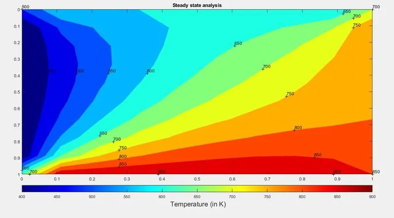
Here we can see that the equations have converged for three of the iteration methods and the contour plot shown above is got.From this contour plot we can understand the conduction of heat from each boundary after the system of equation converged.

Also we can see that the number iterations taken to solve using SOR method is significantly lower compared to other two methods.

For transient state ,

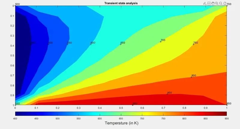
Here we can see that the equations have converged for both explicit and implicit methods and the contour plot shown above is got. From this contour plot we can understand the conduction of heat from each boundary after the system of equation converged.

Compared to steady state the number of iterations required to converge the transient state is very large.

Also we can see that the number iterations taken to solve using SOR method for implicit solver is significantly lower compared to other iterative methods.

CONCLUSION

The Steady state analysis & Transient State analysis on 2D heat conduction equation by using the point iterative techniques has been performed successfully using MATLAB programming and the results have been plotted.