Week 9 - FVM Literature Review

Finite Volume Method (FVM)

FVM is a discretization method for the approximation of partial differential equations based on the integral form of the conservation equations.

In this method a finite volume is considered at each node. This volume defines a control volume. This control volume can be fixed in space or moving with the fluid.

Representation of a control volume is shown below,

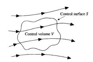
Here control surface is defined as the closed surface which bounds the volume.

Such control volumes are placed at each node as shown below,

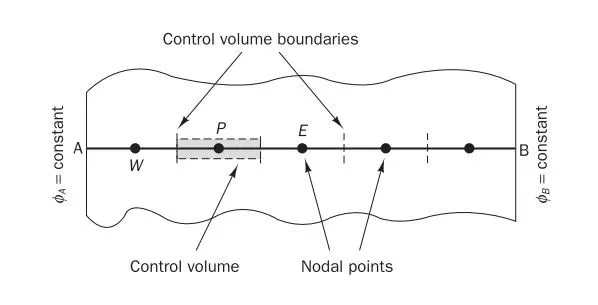
Here we can see that the domain is divided into discrete control volumes. The boundaries of control volumes are positioned mid way between adjacent nodes.

The integration of this control volume expresses the exact conservation of relevant properties for each finite size cell. And hence the discretized equation has a clear physical interpretation.

The conservation of a general flow variable within a finite control volume can be expressed as a balance between the various process tending to increase or decrease it.

Example for FVM

Let us take the one dimensional steady state heat conduction equation,

`d/(dx)(k(dT)/(dx))+S=0`

Consider an insulated rod whose ends are maintained at constant temperatures , thermal conductivity and cross-sectional area are also constant.

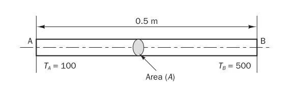
Now we have to find the steady state temperature in the rod. For that let us assume there is no source term(S) present.

Then the equation becomes ,

`d/(dx)(k(dT)/(dx))=0`

We will generate a grid as shown below,

Now we have to integrate the governing equation over a control volume to yield a discretised equation at its nodal point P (center of the control volume chosen).

`intd/(dx)(k(dT)/(dx))dV = (kA(dT)/(dx))_e- (kA(dT)/(dx))_w = 0` Eq---(1)

Here we will apply linear interpolation to find the values of interface diffusion coefficients `k_e` and `k_w` ,

`k_w = (k_W+k_P)/2`

`k_e = (k_P+k_E)/2`

And we will use central differencing scheme to find the diffusive flux terms at east and west face of the control volume.

`((dT)/(dx))_e = (T_E - T_P)/(deltax_(PE))`

`((dT)/(dx))_w= (T_P - T_W)/(deltax_(WP)`

Substituting these values of diffusion coefficient and diffusive flux terms in Equation (1) , we get,

`((k_eA_e)/(deltax_(PE))+(k_wA_w)/(deltax_(WP)))T_P = ((k_wA_w)/(deltax_(WP)))T_W + ((k_eA_e)/(deltax_(PE)))T_E` ---Eq(2)

So the discretised equation for nodes 2,3 & 4 is ,

`a_PT_P=a_WT_W+a_ET_E`

Where , `a_W = k/(deltax)A` , `a_E = k/(deltax)A` and `a_P = a_W+a_E`.

Here , `k_e=k_w=k` , `deltax` and `A_e=A_w=A` are constants.

If we include source term to equation (2) , it will become,

`((k_eA_e)/(deltax_(PE))+(k_wA_w)/(deltax_(WP))-S_P)T_P = ((k_wA_w)/(deltax_(WP)))T_W + ((k_eA_e)/(deltax_(PE)))T_E +S_U` ---Eq(3)

Here `S_u+S_PT_P` represents the source term.

Now we will find the discretised equations for boundary nodes 1 & 5.

For boundary node 1 ,

`((kA)/(deltax)+(2kA)/(deltax))T_P = 0*T_W+((kA)/(deltax))T_E + ((2kA)/(deltax))T_A`

Comparing this equation to Eq(3) we get,

`a_PT_P=a_WT_W+a_ET_E+S_u`

Where , `a_W = 0` , `a_E = k/(deltax)A` and `a_P = a_W+a_E-S_P` , `S_P = -(2kA)/(deltax)` and `S_u =(2kA)/(deltax)T_A`

Similarly we can find the discretised equation for boundary node 5 given below,

`a_PT_P=a_WT_W+a_ET_E+S_u`

Where , `a_W = k/(deltax)A` , `a_E =0` and `a_P = a_W+a_E-S_P` , `S_P = -(2kA)/(deltax)` and `S_u =(2kA)/(deltax)T_B`

Now we have to substitute the values of `k`,`A`,`deltax`, boundary conditions `T_A` & `T_B` and we will get a set of linear algebraic equations. Solving these equations will give us the steady state temperature distribution in the rod.

FVM Vs FDM

Finite Difference Method (FDM) is a discretization technique in which the partial derivatives of the governing equations are replaced by approximate algebraic difference quotients, where the algebraic difference quotients are expressed in terms of the flow-field variables at two or more of the discrete grid points.

The major differences between FVM and FDM are as follows,

1. In FVM , integral form of the governing equations are used , where as in FDM differential form of the governing equations are used.
2. FDM need structured grid points where as FVM can have unstructured grid points.
3. FVM always satisfies the conservation laws where as FDM does not.
4. FVM can be used for complex geometries but FDM cannot be used in such scenarios.
5. FDM can have higher order functions easily but in case of FVM the functions cannot be easily made of higher order.

Interpolation schemes

The approximations to the integrals require the values of the variables at locations other than computational nodes (i.e control volume centers) and to get those values we need to use different interpolation schemes.

Some of the interpolation schemes are Upwind Interpolation Scheme (UDS) , Linear Interpolation(CDS) , Quadratic Upwind Interpolation for Convective Kinematics (QUICK) etc….

Flux limiters

These are used to make a scheme satisfy the conditions to be TVD scheme. To better understand this we have to know about TVD.

TVD stands for Total Variation Diminishing , it is a type of high resolution scheme formulated to overcome the issue of oscillatory behaviour found in higher order numerical schemes when solving flow fields with discontinuities like shock waves. Any numerical scheme that gives rise to such oscillations does not satisfy the TVD condition.

TVD condition states,

`TV(phi^(n+1))<=TV(phi^n)` , where `TV` represents the integrated quantity called Total Variation , `n` & `n+1` represents consecutive time steps.

This condition basically means that the total variation of the discrete solution should diminish with time.

To make other numerical schemes to satisfy this TVD condition , we have to multiply the flux terms by a non-linear function. These functions should be formed such that it forces the difference equations to satisfy the TVD condition.

These non-linear term is represented by `Psi` ,

`Psi = Psi(r)` , where ‘`r`’ is the non-linear function

The condition for a scheme to be TVD on the basis of `r"-"Psi` relationship is as follows,

• If `0 then `Psi(r)<=2r`
• If `r>=1` then `Psi(r)<=2`

But the numerical schemes except for upwind difference does not satisfy the above conditions. So in order to make those schemes TVD we have to limit the possible values of the flux term.

Now the `Psi(r)` term is called the flux limiter function , because it will limit the flux values. A flux limiter will restrict the amplitude of the gradient appearing in the original higher order numerical schemes.