Week 1- Mixing Tee

AIM

To set up steady-state simulations to compare the mixing effectiveness when hot inlet temperature is 36°C & the Cold inlet is at 19°C for a mixing tee problem using ANSYS software.

The two cases to be simulated are as follows,

• Case 1:- Short mixing tee with a hot inlet velocity of 3m/s and momentum ratio of 2 & 4.
• Case 2:- Long mixing tee with a hot inlet velocity of 3m/s and momentum ratio of 2 & 4.

Use k-epsilon & k-omega SST turbulence model for the first case and select the suitable model for further cases.

GOVERNING EQUATIONS

Temperature of the mixture is given by,

`T_(mixture)=(m_(hot)*T_(hot)+m_(cold)*T_(cold))/(m_(hot)+m_(cold))`

Where , ‘T’ is the temperature of the fluid and ‘m’ is the mass flow rate.

`m = rhoAv`

Where , `rho` is the density of the fluid , `A` is the cross-sectional area and ‘`v`’ is the velocity of the fluid.

`"Momentum ratio" = ("velocity at the cold inlet")/("velocity at the hot inlet")`

OBJECTIVE

1. To compare the cell count , average outlet temperature and number of iterations for convergence for the given two case studies.
2. To perform mesh independent study for any one of the case study.
3. To use contour & line plots to study the output values of velocity and temperature along and across the length of the pipe.

THEORY

• Mixing tees:- They are basically T-junctions in which two fluid streams with different physical or chemical properties mix together. An example for this type of setup is shown below,

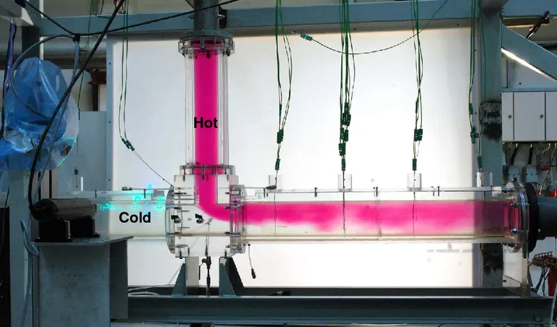
The mixing of the fluids at two different temperatures takes place at the T-junction as shown in diagram. At the outlet we get the mixture of these two fluids at the required temperature.

The CFD simulations of such setup are very important in practical applications like nuclear reactors. As when there is a large temperature difference between two fluid streams , large temperature fluctuations can occur, which will lead to thermal fatigue of the piping system. Especially in case of these tee connections temperature mixing effects cannot be accurately monitored by the mechanical instrumentations.

• Turbulence model:- It is the mathematical model to predict the effects of turbulence. One of the most commonly used models is RANS , which stands for Reynolds-Averaged Navier Stokes model. The k-ε and k-ω models comes under the RANS models of two equation type. The two equation type RANS models contain two transport equations for two turbulence properties ,which are turbulence kinetic energy (k) and the dissipation rate of turbulence kinetic energy (ε) or the specific dissipation rate (ω). The k-ε model has a modified version called realizable k-ε and similarly the k-ω model has a more advanced version called k-omega Shear Stress Transport (SST) model.

SIMULATION CONDITIONS

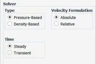
The solver used for the simulation is pressure based and of steady state type as the simulations are to be performed for steady state condition.

Fluid :- air

Density `= 1.225 (Kg)/m^3`

Velocity at the hot inlet = 3m/s

For momentum ratio `= 2`,

`"velocity at the cold inlet" = "velocity at the hot inlet" * "momentum ratio"`

`= 3 *2 = 6` m/s

For momentum ratio `= 4`,

velocity at the cold inlet `= 3 * 4 = 12` m/s

Temperature at the hot inlet `= 36°C`

Temperature at the cold inlet `= 19°C`

Pressure at the outlet `= 1` atm

Initialization method :- Hybrid

PROCEDURE (CASE 1)

• In this case the short mixing tee geometry will be used , whose dimensions are shown below,

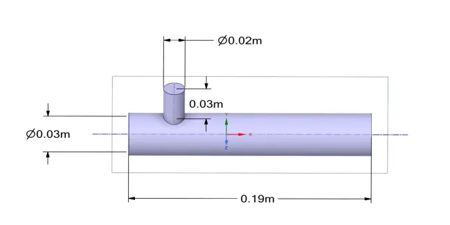
This geometry is processed using the Space-Claim software.

• The mesh is generated for this geometry using the ANSYS meshing software. The element size is kept at the default value of 10.219mm . The meshed geometry is shown below with its element qualities,

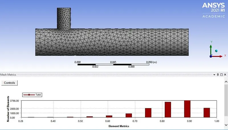
• From the element quality chart , it can be seen that most of the elements have quality greater than 0.6 and hence the meshed geometry is of acceptable quality.
• Different parts of the geometry are named as per the requirements.
• Using the ANSYS FLUENT software the simulation parameters are defined.
• For the physics of the fluid energy equations are used.

To select the turbulence model, the simulation has to be run using both realizable k-ε and k-ω SST models.

Let the momentum ratio used for this be 2.

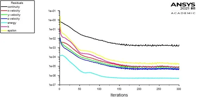
First let us do the simulation for realizable k-ε model for 300 iterations. The simulation result showing the residual values is given below ,

Now the viscous model is changed to k-ω SST model and the simulation is run for 450 iterations. The simulation result showing the residual values is given below ,

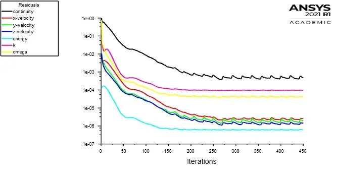
On comparing the above two results , it is clear that the number of iterations for convergence for realizable k-ε model is less than that of k-ω SST model. The former took only 160 iterations to attain stability where as the latter took almost 250 iterations. And hence we will use realizable k-ε for simulation.

Note :- From here on the viscous model used for the simulations will be realizable k-ε model.

• For output plots , an area weighted average report is created for the outlet temperature.
• The simulation is done for momentum ratio 2 & 4.
• In the CFD post software the simulation results are post processed.
• Contour and line plots in the XY plane and ZX plane will be made.
• In the XY plane plots will be made in the center of the pipe and in the ZX plane the plots will be made for the region just after the T-junction.

PROCEDURE (CASE 2)

• In this case the long mixing tee geometry will be used , whose dimensions are shown below,

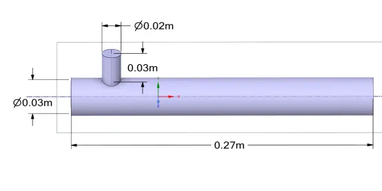
This geometry is processed using the Space-Claim software.

• In the ANSYS meshing software , the mesh is generated and the parts of the geometry is named as per the requirement.

Mesh Independent Test

• The mesh independent test will be performed for this case to ensure that the simulation output values are independent of the mesh size.

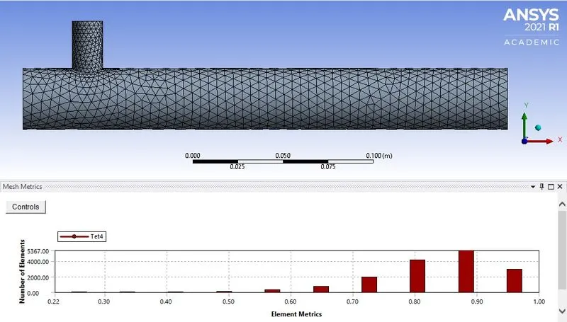
The test will be done for three element sizes which will be of coarse , medium and fine type. For the coarse type the element size used will the default value.

These meshes and their quality are shown below,

Coarse mesh,

Medium mesh,

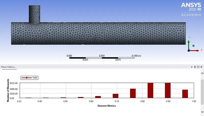
Fine mesh,

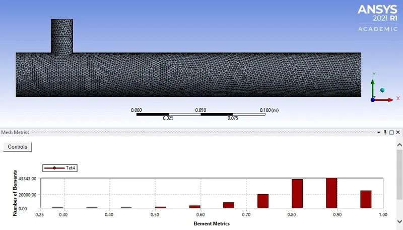
The simulation will be done for all three mesh sizes and the percentage change in outlet temperature value will be recorded after each refinement. All three simulations are done for momentum ratio 2.

As already mentioned the viscous model used will be k-ε model.

• The result of these simulations are shown in the table given below,

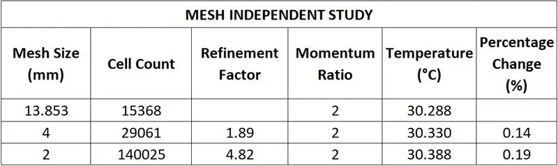
The percentage change after each mesh refinement is less than 0.2 % which is enough to say that the simulation output values are independent of the mesh size.

Also from the results it is clear that as the mesh is refined we get slightly accurate results. Hence the finest mesh will be used for further simulations.

• The finest element size will be used for the simulations for momentum ratio 4.
• For output plots , an area weighted average report is created for the outlet temperature.
• After the simulation is done for momentum ratios 2 & 4, the simulation results will be post processed using the CFD post software.
• Contour and line plots in the XY plane and ZX plane will be made.
• In the XY plane plots will be made in the center of the pipe and in the ZX plane the plots will be made for the region just after the T-junction.

RESULTS

CASE 1 (short mixing tee)

For momentum ratio 2 ,

Convergence plot,

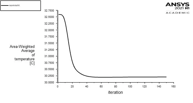
Average outlet temperature plot,

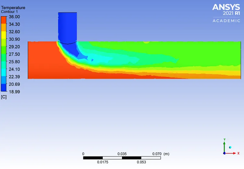
Temperature contour plot along the pipe,

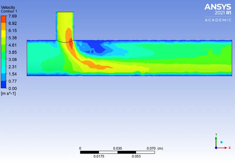
Velocity contour plot along the pipe,

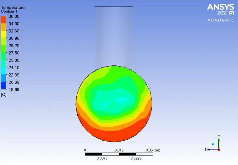
Temperature contour plot across the pipe,

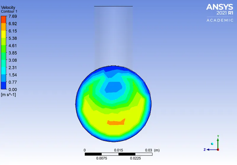
Velocity contour plot across the pipe,

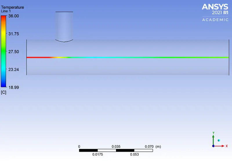
Temperature line plot along the pipe,

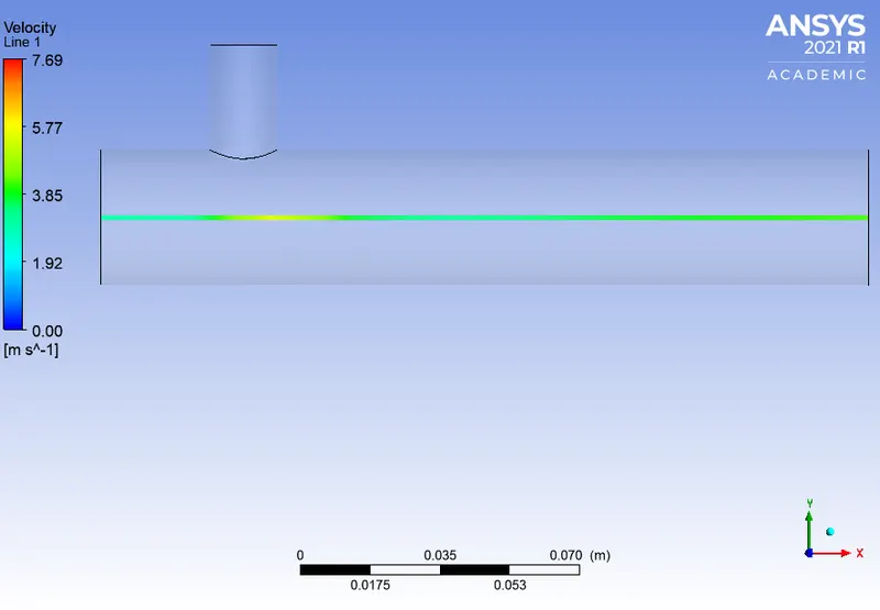
Velocity line plot along the pipe,

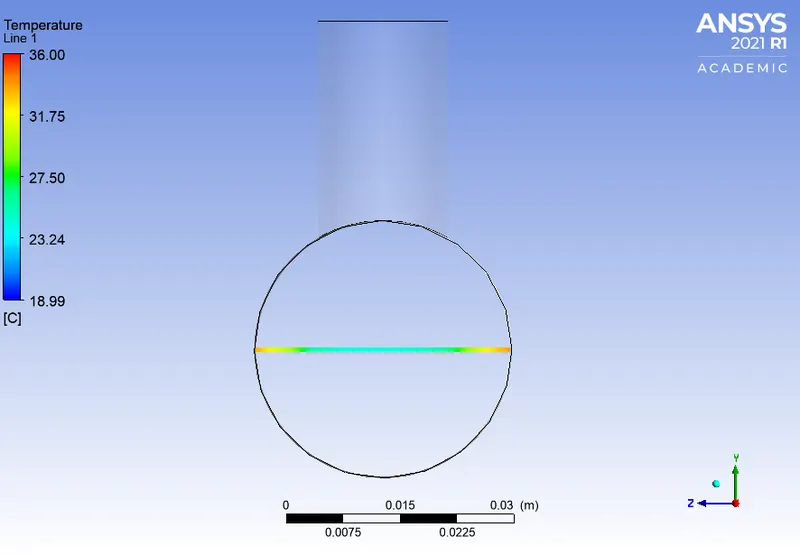
Temperature line plot across the pipe,

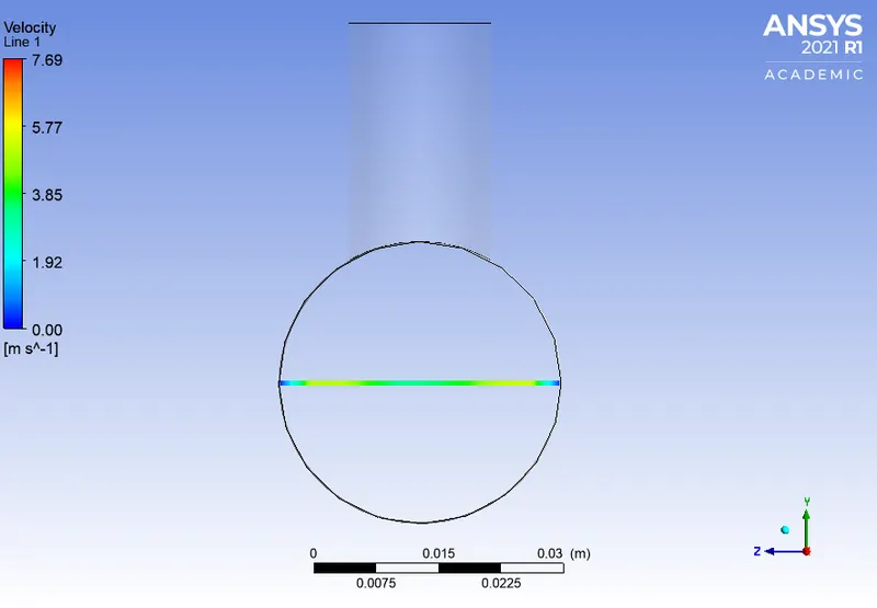
Velocity line plot across the pipe,

For momentum ratio 4 ,

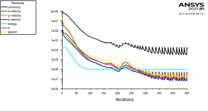
Convergence plot,

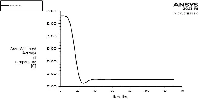
Average outlet temperature plot,

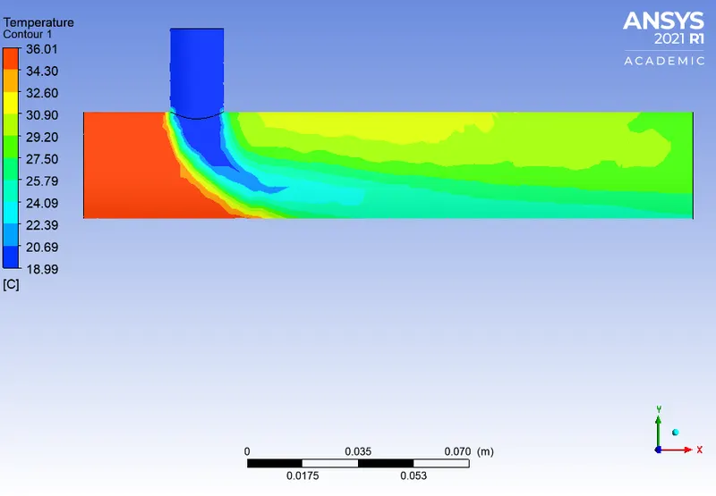
Temperature contour plot along the pipe,

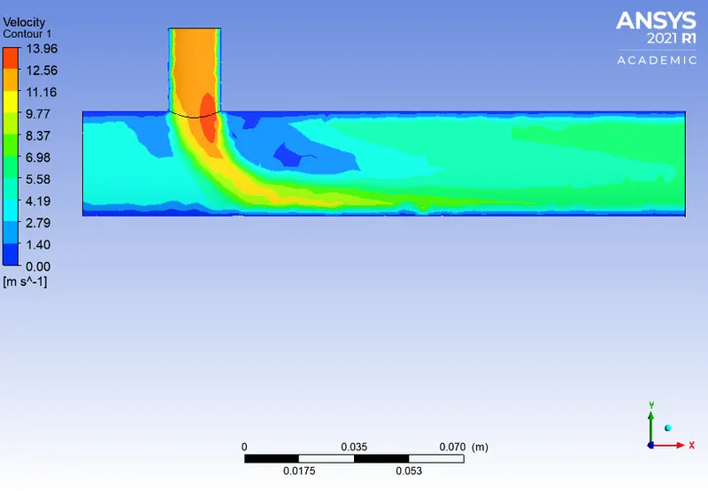
Velocity contour plot along the pipe,

Temperature contour plot across the pipe,

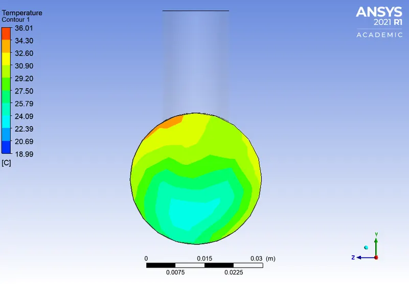
Velocity contour plot across the pipe,

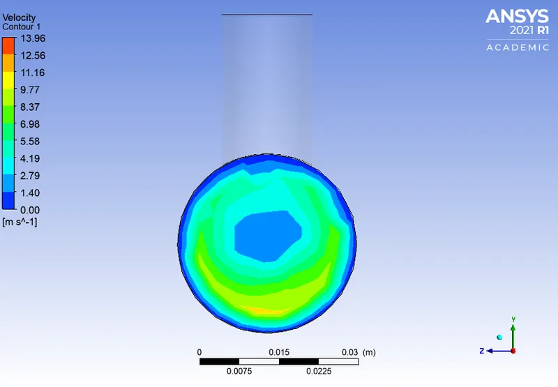
Temperature line plot along the pipe,

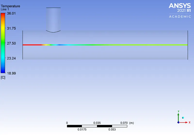
Velocity line plot along the pipe,

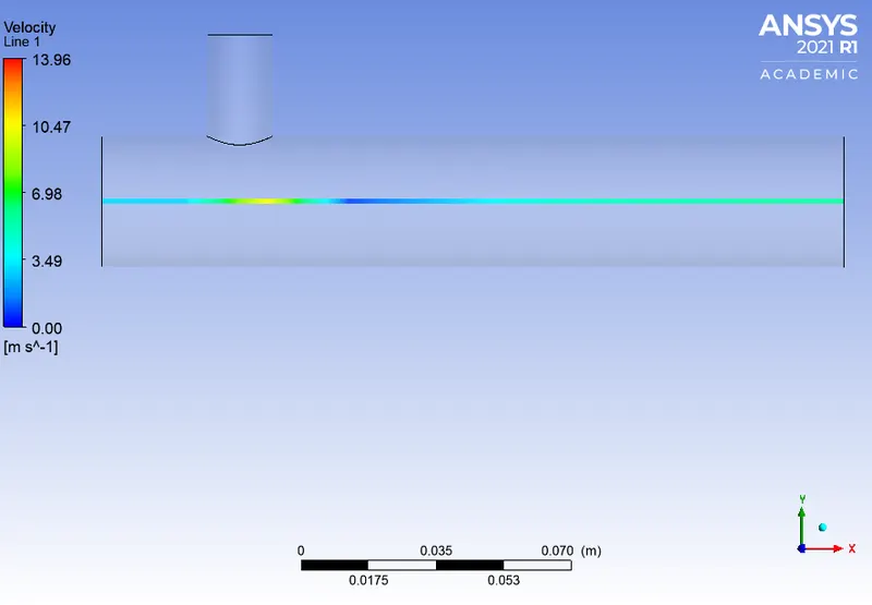
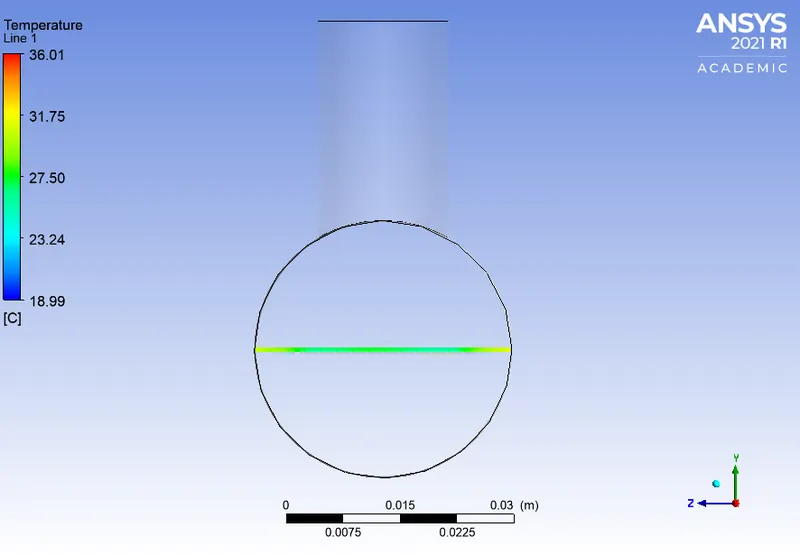
Temperature line plot across the pipe,

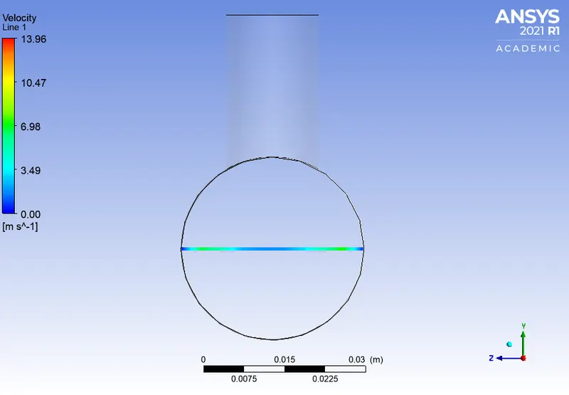
Velocity line plot across the pipe,

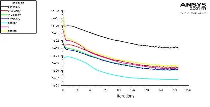
CASE 2 (long mixing tee)

For momentum ratio 2 ,

Convergence plot,

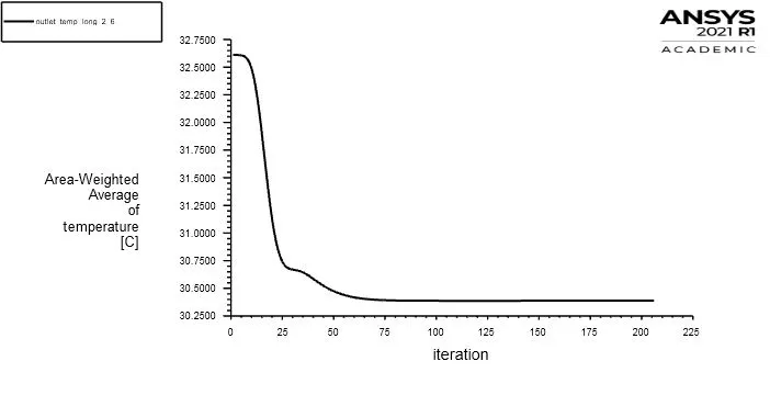
Average outlet temperature plot,

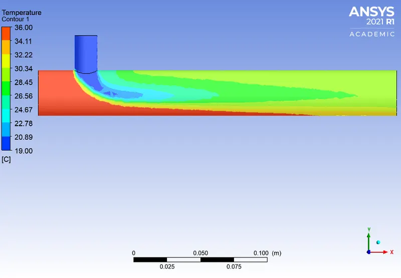
Temperature contour plot along the pipe,

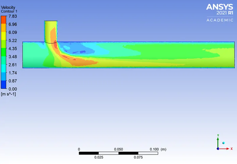
Velocity contour plot along the pipe,

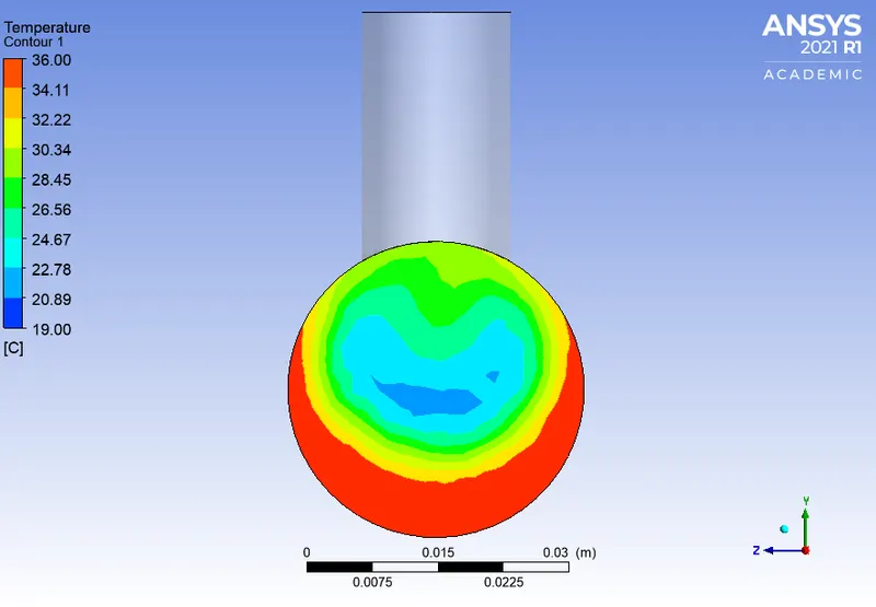
Temperature contour plot across the pipe,

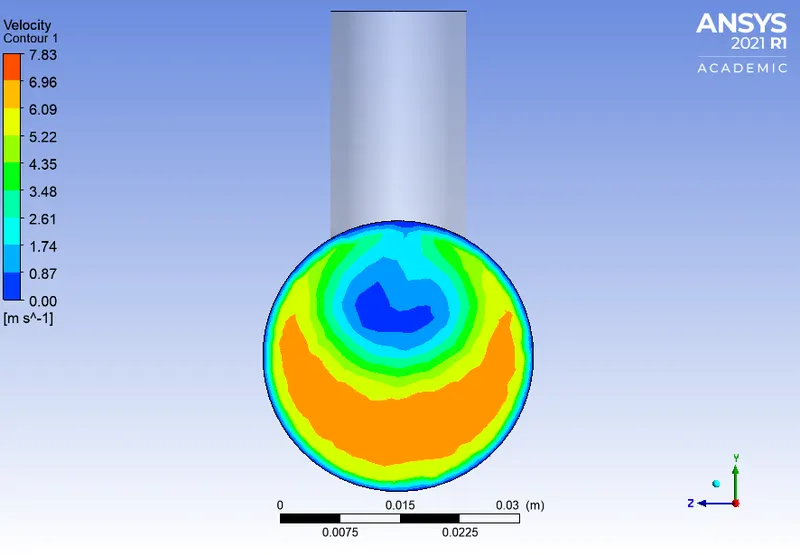
Velocity contour plot across the pipe,

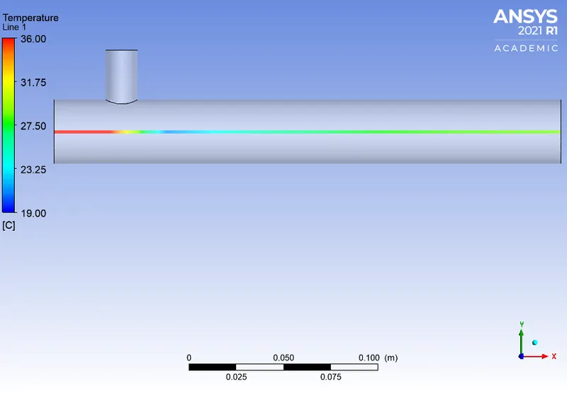
Temperature line plot along the pipe,

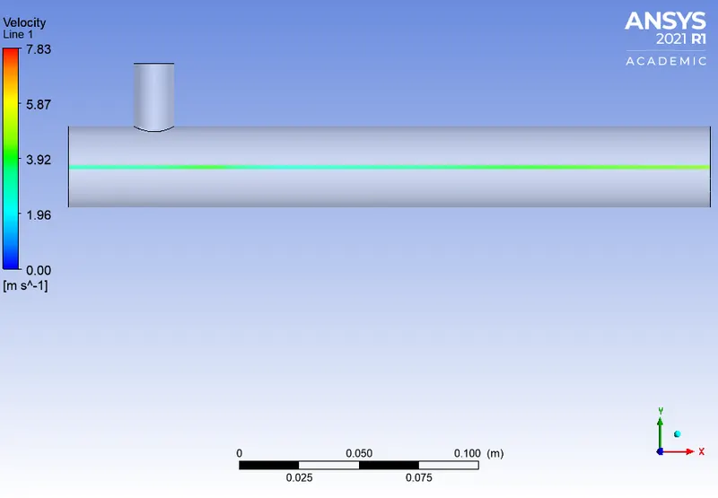
Velocity line plot along the pipe,

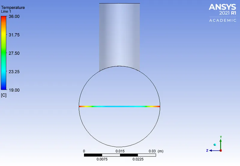
Temperature line plot across the pipe,

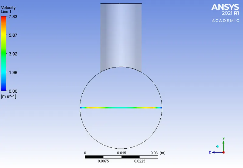
Velocity line plot across the pipe,

For momentum ratio 4 ,

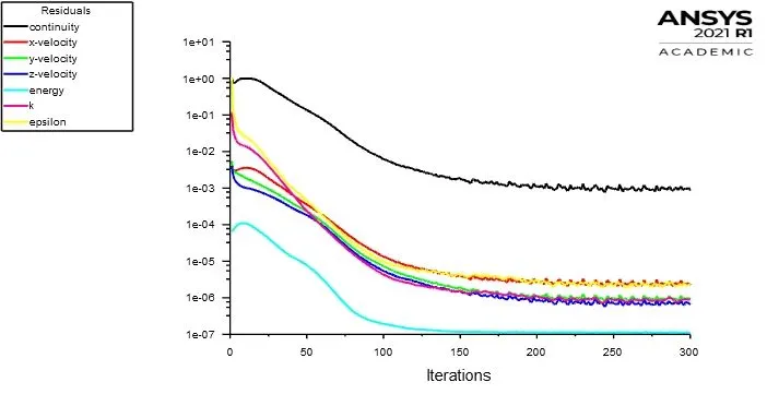
Convergence plot,

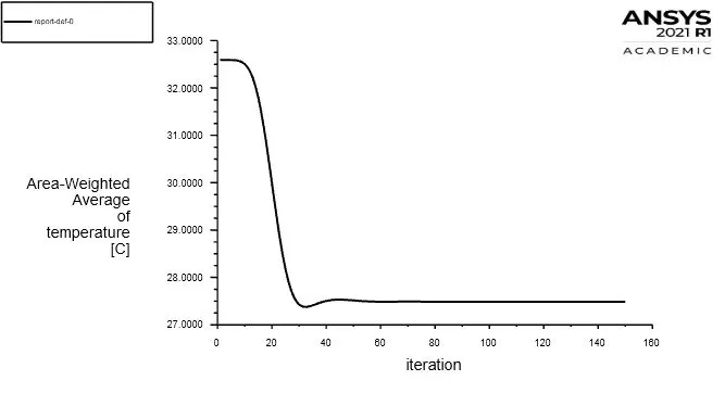
Average outlet temperature plot,

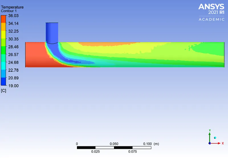
Temperature contour plot along the pipe,

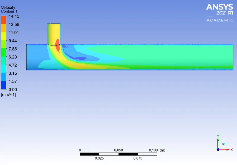
Velocity contour plot along the pipe,

Temperature contour plot across the pipe,

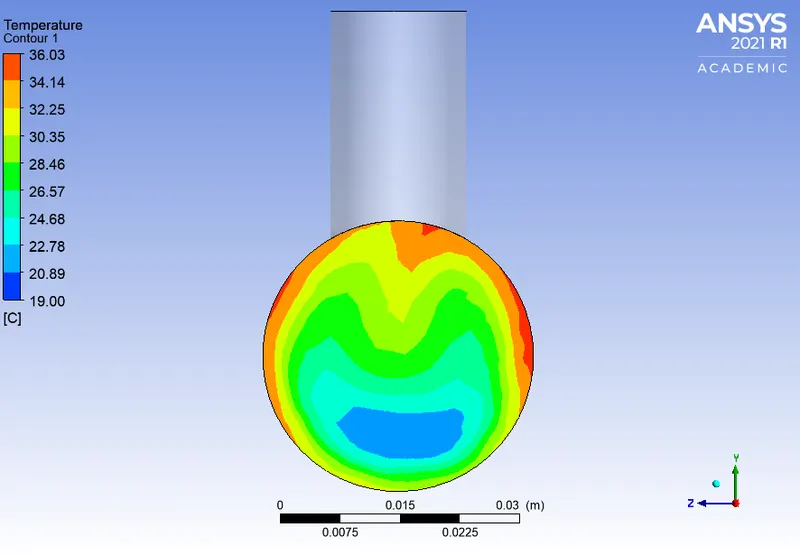
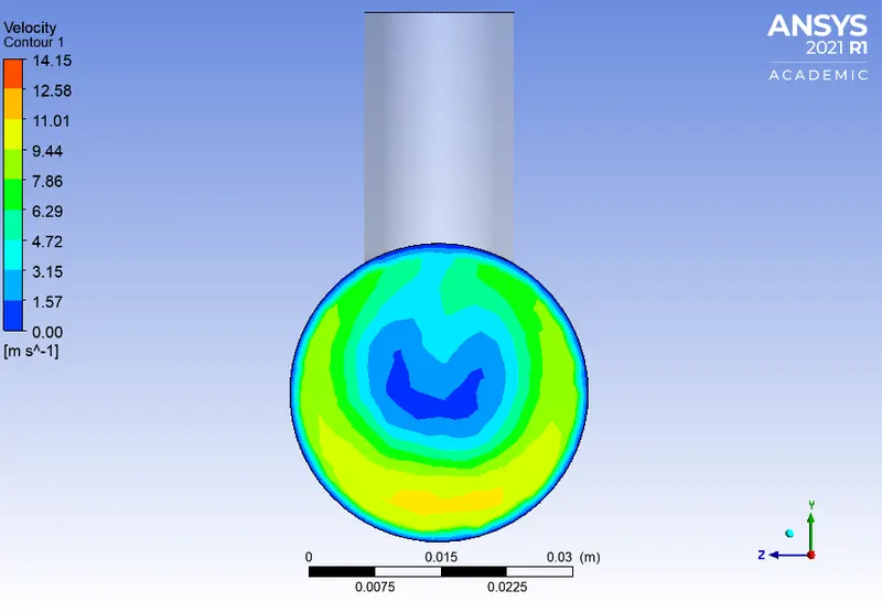
Velocity contour plot across the pipe,

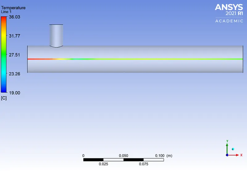
Temperature line plot along the pipe,

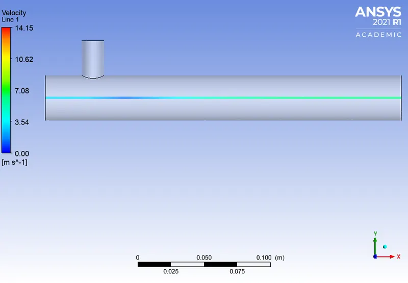
Velocity line plot along the pipe,

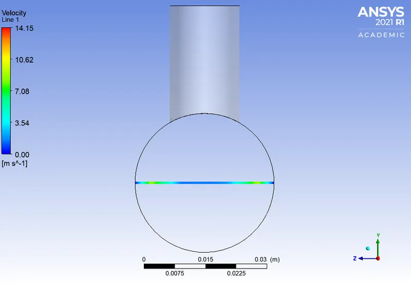
Temperature line plot across the pipe,

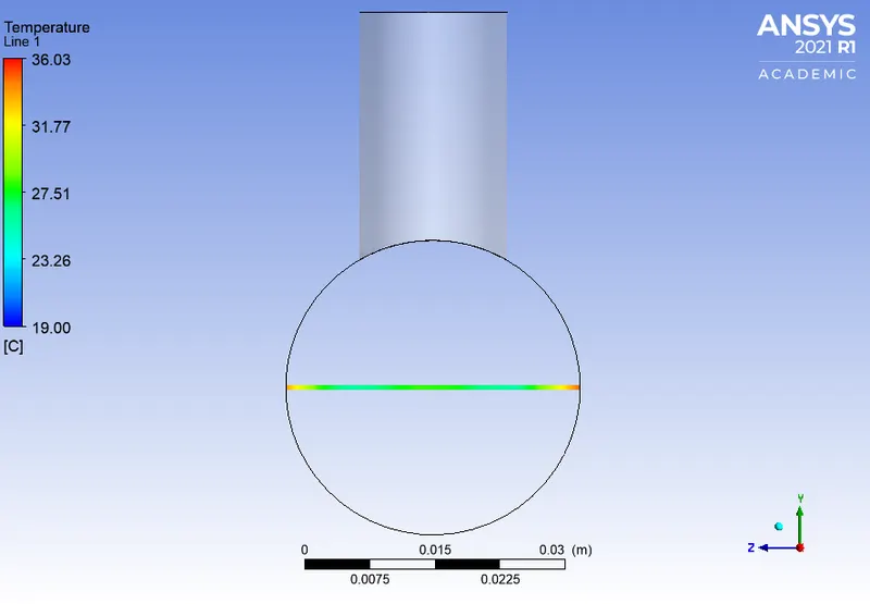
Velocity line plot across the pipe,

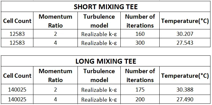
The comparison between the output results of short mixing tee and long mixing tee is done in the table given below,

VALIDATION

The simulation results can be validated using the formula for temperature of the mixture of fluid.

For that mass flow rate of the two fluids has to be calculated.

For hot fluid,

`m_(hot) = rhoAv_(hot)`

`A=pi(d^2/4)`

`d=0.0339m`

`A= pi*(0.0339^2/4) = 9.026*10^-4 m^2`

`m_(hot) = 1.225*9.026*10^-4*3 = 3.317*10^-3 (Kg)/s`

For cold fluid at momentum ratio 2,

`m_(cold) = rhoAv_(cold)`

`A=pi(d^2/4)`

`d=0.017m`

`A= pi*(0.017^2/4) = 2.27*10^-4 m^2`

`m_(cold) = 1.225*2.27*10^-4*6 = 1.668*10^-3 (Kg)/s`

For cold fluid at momentum ratio 4,

`m_(cold) = rhoAv_(cold)`

`A=pi(d^2/4)`

`d=0.017m`

`A= pi*(0.017^2/4) = 2.27*10^-4 m^2`

`m_(cold) = 1.225*2.27*10^-4*12 = 3.34*10^-3 (Kg)/s`

Temperature of the mixture at momentum ratio 2,

`T_(mixture) = ((3.317*10^-3*36)+(1.668*10^-3*19))/(3.317*10^-3+1.668*10^-3)`

`=(0.1194+0.031692)/0.004985`

`=30.31°C`

Temperature of the mixture at momentum ratio 2,

`T_(mixture) = ((3.317*10^-3*36)+(3.34*10^-3*19))/(3.317*10^-3+3.34*10^-3)`

`=(0.1194+0.06346)/0.006657`

`=27.47°C`

These results are tabulated below ,

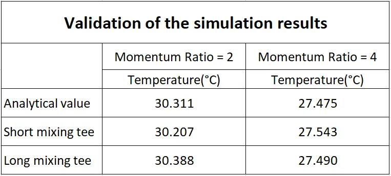
From these results it is clear that the simulation results are very close to analytical values and hence it can be concluded that the simulation results are accurate.

CONCLUSION

The steady state simulation to compare the mixing effectiveness of fluids at different temperatures in a mixing tee junction has been done successfully using ANSYS software and the results has been validated.

From those results following conclusions can be made,

The temperature close to the pipe wall in both the cases are higher than that towards the center of the pipe and this can be seen in the contour plots of the same.

And the velocity of the fluid near to the pipe wall is minimum and it is highest towards the center of the pipe.

As the momentum ratio value increases the average temperature value at the outlet has decreased by almost 3°C. So it could be concluded that the momentum ratio is inversely proportional to the average temperature value at the outlet. If the average outlet temperature required is low , the velocity of the cold fluid has to be increased.

The effect of length on the outlet temperature is quite negligible in this scenario as the temperature values are close to each other in both the cases. And hence it could be concluded that the length of the pipe does not make huge difference in the average outlet temperature value.