Week 11 - Simulation of Flow through a pipe in OpenFoam
AIM
To simulate an axi-symmetric flow by applying the wedge boundary condition using OpenFOAM software. The conditions for the simulation is as follows,
- The flow is laminar and flows through a constant cross-section pipe at an inlet Reynold’s number of 2100.
- The simulation can be transient or steady state.
- Validate the results with the Hagen- Poiseuille's equations for the fully developed flow.
THEORY
Laminar flow is a type of fluid flow which is characterized by smooth streamlines and highly ordered motion. Such a flow is seen when highly viscous fluids like oils flows in small pipes or narrow passages.
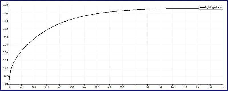
Hydrodynamic entry length is defined as the distance from the pipe entrance to where the wall shear stress reaches within about 2 percent of the fully developed value. Here the fully developed region is where the velocity profile remains unchanged.
The flow field depends mainly on Reynolds number , which is defined as the ratio of inertial forces to viscous forces. It is represented by ‘Re’.
GOVERNING EQUATIONS
The Hagen- Poiseuille's equations for a fully developed laminar flow are given below ,
The hydrodynamic entry length , `L_h cong 0.06*Re*D`
Where `Re` is the Reynolds number and `D` is the diameter of the pipe.
Average velocity of the flow , `V_(avg) = (nu*Re)/D`
Where `nu` is the kinematic viscosity (`nu = mu/rho`)
Maximum velocity , `u_(max) = 2*V_(avg)`
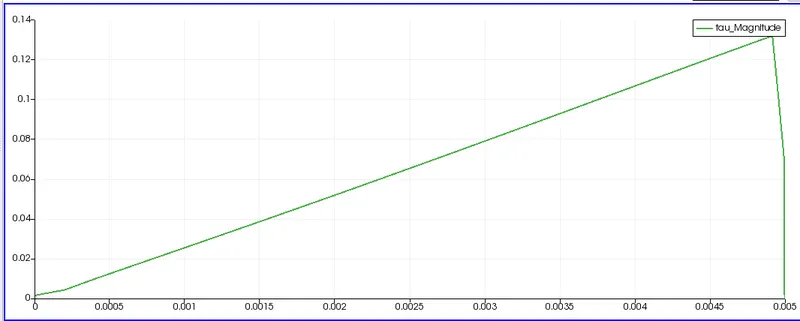
Maximum shear stress , `tau_(max) = (2*mu*u_(max))/R`
Where `mu` is the dynamic viscosity and `R` is the radius of the pipe.
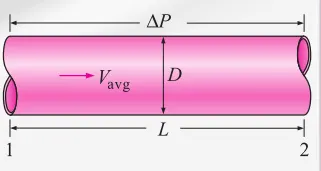
Pressure drop , `DeltaP = (32*mu*L*V_(avg))/D^2`
Where L is the distance between the two pressures measured at point 1 and point 2 as shown in the diagram given below,
OBJECTIVE
- To write a code in MATLAB to automate the generation of blockMeshDict file.
- To validate Hydro-dynamic length with the numerical result.
- To validate the fully developed flow velocity profile with its analytical profile.
- To validate maximum velocity and pressure drop for fully developed flow.
- To post-process shear stress and validate wall shear stress for fully developed flow.
ASSUMPTIONS
Here we have assumed the fluid to be water at `25^circ C`. The density of the water at this temperature is `997 (Kg)/m^3` , dynamic viscosity is `8.891"*"10^-4 (Kg)/(ms)` and kinematic viscosity is `8.917"*"10^-7 m^2/s`.
PROCEDURE
- First let us write a code in MATLAB to create the blockMeshDict file. The script file is given below,
clear all close all clc % input values d= input('enter the diameter of the pipe : '); Re = input('enter the Reynolds number : '); theta=input('enter the wedge angle : '); nu = input('enter the kinematic viscosity of the fluid : '); rho = input('enter the density of the fluid : '); % total length of the pipe = hydrodynamic length + fully developed region l = (0.06*Re*d)+340; % radius of the pipe r=d/2; %% creating the blockMeshDict file f1=fopen('blockMeshDict.txt','w'); % unit=input('enter conversion to meter value : ') fprintf(f1,'FoamFile\n{\nversion 2.0;\nformat ascii;\nclass dictionary;\nobject blockMeshDict;\n}\n\n'); fprintf(f1,'convertToMeters %f;\n\n',0.001); % vertices fprintf(f1,'vertices\n(\n'); fprintf(f1,' (%f %f %f)\n', 0,0,0) ; fprintf(f1,' (%f %f %f)\n', l,0,0) ; fprintf(f1,' (%f %f %f)\n', l, r*cosd(theta/2),-r*sind(theta/2)) ; fprintf(f1,' (%f %f %f)\n', 0, r*cosd(theta/2),-r*sind(theta/2)); fprintf(f1,' (%f %f %f)\n', l, r*cosd(theta/2),r*sind(theta/2)) ; fprintf(f1,' (%f %f %f)\n', 0, r*cosd(theta/2),r*sind(theta/2)); fprintf(f1,');\n\n'); % blocks fprintf(f1,'blocks\n(\n'); fprintf(f1,' hex (%g %g %g %g %g %g %g %g)', 0 ,1,2,3,0,1,4,5); fprintf(f1,' (%g %g %g) simpleGrading (1 0.2 1)\n);\n\n', 300 , 50 ,1); % edges fprintf(f1,'edges\n(\n'); fprintf(f1,' arc 3 5 (0 %f 0)\n',r); fprintf(f1,' arc 2 4 (%f %f 0)\n',l,r); fprintf(f1,');\n\n'); % boundary fprintf(f1,'boundary\n(\n inlet\n {\n type patch;\n faces\n (\n (3 0 0 5)\n );\n }\n\n'); fprintf(f1,' outlet\n {\n type patch;\n faces\n (\n (2 4 1 1)\n );\n }\n\n'); fprintf(f1,' front\n {\n type wedge;\n faces\n (\n (5 0 1 4)\n );\n }\n\n'); fprintf(f1,' back\n {\n type wedge;\n faces\n (\n (3 2 1 0)\n );\n }\n\n'); fprintf(f1,' top\n {\n type wall;\n faces\n (\n (2 3 5 4)\n );\n }\n\n'); fprintf(f1,' bottom\n {\n type empty;\n faces\n (\n (0 1 1 0)\n );\n }\n'); fprintf(f1,');\n\n'); fclose(f1); %% %input value of section between which pressure drop is measured L = input(' enter length of the pipe section (pressure drop) : ' ); % Analytical values for validating the simulated results fprintf('\n\n Analytical values\n') % Inlet velocity calculation v_avg = (nu*Re)/(d*10^-3); u_max = 2*v_avg; fprintf(' The average velocity is %f m/s \n',v_avg) fprintf(' The maximum velocity is %f m/s \n',u_max) % maximum stress tau_max = (2*nu*rho*u_max)/(r*10^-3); fprintf(' The maximum shear stress is %f N/m^2',tau_max) % Pressure drop delta_P = (32*L*rho*nu*v_avg)/(d*10^-3)^2; fprintf(' \n The pressure drop is %f N/m^2 \n',delta_P) %Hydrodynamic length L_h = (0.06*Re*d*10^-3); fprintf(' The Hydrodynamic length is %f m \n',L_h)
The steps involved are given below,
- The values which has to be input by the user are defined. Then using this some more parameters are calculated like length of the pipe and radius of the pipe.
- Now we will create a file named blockMeshDict using ‘fopen’ command. Then we will write into this file.
- Opening part of the file is written as it is and then the conversion to meter value is defined. This value specifies the multiplication factor using which we can convert the numbers used in the file to meters. If we use millimeters to define the geometry then the conversion factor will be 0.001 .
- Next we have to specify the vertices of the geometry. Since we are creating a wedge geometry , it will run along the center line of one of the coordinate axis and will straddle that axis. This wedge geometry and its vertices are shown in the diagram given below,
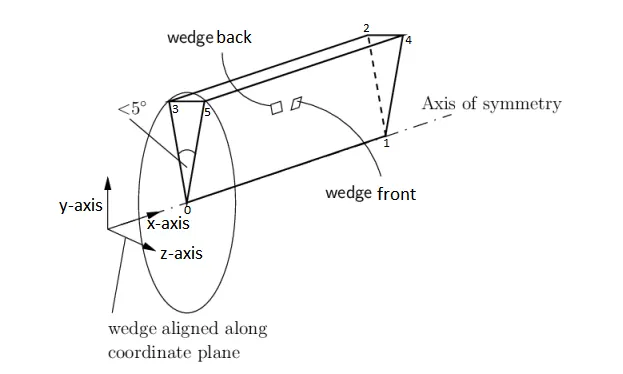
- The coordinate values of vertices 2,3,4 & 5 are calculated by using trigonometry. Let the face of the wedge at x=0 is shown below,
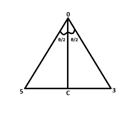
In this triangle the length of the side from 0 to 3 and 0 to 5 is equal to the radius of the pipe. We have to find the length of the side 0 to C , 3 to C and 5 to C. This can be found out by applying trigonometric formulas. Here `theta` is the wedge angle. By finding out those lengths we get the coordinate values of those vertices. The same procedure is done for the wedge face on the other end of the x-axis.
- Next we have defined the block , which here is the wedge geometry. Since blocks has to be defined using 8 vertices , we will enter the vertices 0 and 1 two times. This basically represents a geometry with one of its faces collapsed. And we have used a grid with 300 cells on the x-axis , 50 cells along the y-axis and 1 cell in z-axis. Grading has been given for mesh along y-axis , the grading factor is 0.2 .
- After that the edges are created , which will form the arc required for the geometry. Here we have to specify the vertices between which we need an arc. So in this case it is 3 & 5 and 2 & 4. Then a point through which the arc passes has to be mentioned. In this case the point is the radius of the pipe.
- Next we have defined the boundaries and their types. Here the wedge front and back side has to be the type wedge itself. And another thing to note is that the bottom part (block face of zero area) has to be of type empty.
- Now the file is closed using ‘fclose’ command.
- We will also include analytical calculations inside this program so that we can validate the simulation results after post-processing it by comparing those values to the analytical values.
- After creating the blockMeshDict file , copy it to the OpenFOAM folder and then use the terminal to modify the other files.
- In the controlDict file we have changed the simulation time to 5 seconds and the time step value to 0.01 .
- Next we have to modify the initial conditions of pressure and velocity. We will specify the inlet and outlet values of those two in their respective files named ‘p’ and ‘U’ in the folder ‘0’.
- Here we have to mention type wedge for all those faces which were given type wedge inside the blockMeshDict file. Similarly face with type empty also remains the same.
- Now we will create the block mesh using the ‘blockMesh’ command and then solved using the solver ‘icoFoam’ which isthe transient solver for incompressible, laminar flow of Newtonian fluids.
- After solving we will open the post-processor , paraview using the command ‘paraFoam’.
- Here we will run the simulation and plot the necessary graphs.
- To plot the shear stress we have to first calculate the magnitude of velocity U , and then find the gradient of this velocity. After that this gradient value has to be multiplied with dynamic viscosity of the fluid which gives us the shear stress value. All these calculations are done using built-in calculator of paraview and the gradient is found using Gradient of unstructured dataset tool.
RESULTS
blockMeshDict file,
FoamFile
{
    version     2.0;
    format      ascii;
    class       dictionary;
    object      blockMeshDict;
}
// * * * * * * * * * * * * * * * * * * * * * * * * * * * * * * * * * * * * * //

convertToMeters 0.001000;

vertices
(
     (0.000000  0.000000 0.000000)
     (1600.000000  0.000000 0.000000)
     (1600.000000  4.995241 -0.218097)
     (0.000000  4.995241 -0.218097)
     (1600.000000  4.995241 0.218097)
     (0.000000  4.995241 0.218097)
);

blocks
(
     hex (0 1 2 3 0 1 4 5) (300 50 1) simpleGrading (1 0.2 1)
);

edges
(
     arc 3 5 (0 5.000000 0)
     arc 2 4 (1600.000000 5.000000 0)
);

boundary
(
     inlet
     {
          type patch;
          faces
          (
             (3 0 0 5)
          );
     }

     outlet
     {
          type patch;
          faces
          (
             (2 4 1 1)
          );
     }

     front
     {
          type wedge;
          faces
          (
             (5 0 1 4)
          );
     }

     back
     {
          type wedge;
          faces
          (
             (3 2 1 0)
          );
     }

     top
     {
          type wall;
          faces
          (
             (2 3 5 4)
          );
     }

     bottom
     {
          type empty;
          faces
          (
             (0 1 1 0)
          );
     }
);
Initial pressure file,
FoamFile
{
    version     2.0;
    format      ascii;
    class       volScalarField;
    object      p;
}
// * * * * * * * * * * * * * * * * * * * * * * * * * * * * * * * * * * * * * //

dimensions      [0 2 -2 0 0 0 0];

internalField   uniform 0;

boundaryField
{
    inlet
    {
        type            zeroGradient;

    }

    outlet
    {
        type            fixedValue;
        value           uniform 0;
    }

    front
    {
        type            wedge;
    }

    back
    {
        type            wedge;
    }

    top
    {
    	type 	        zeroGradient;
    }

    bottom
    {
    	type 	        empty;
    }
}
Initial velocity file,
FoamFile
{
    version     2.0;
    format      ascii;
    class       volVectorField;
    object      U;
}
// * * * * * * * * * * * * * * * * * * * * * * * * * * * * * * * * * * * * * //

dimensions      [0 1 -1 0 0 0 0];

internalField   uniform (0 0 0);

boundaryField
{
    inlet
    {
        type            fixedValue;
        value           uniform (0.187257 0 0);
    }

    outlet
    {
        type            zeroGradient;
    }

    front
    {
        type            wedge;
    }

    back
    {
        type            wedge;
    }

    top
    {
    	type 	        noSlip;
    }

    bottom
    {
    	type 	        empty;
    }
}
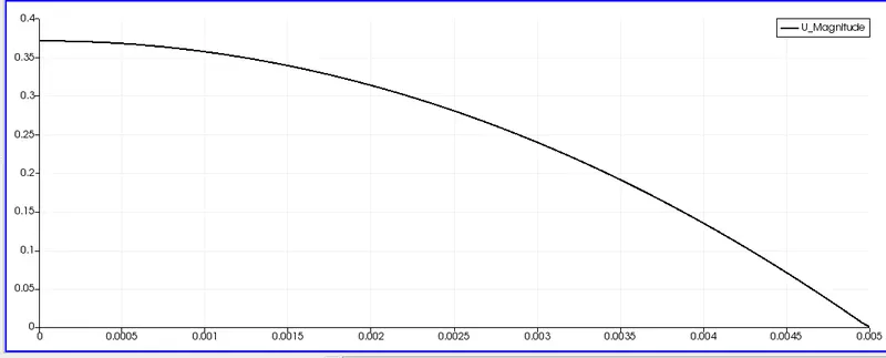
Simulated velocity profile at fully developed region ,
Maximum velocity (at r = 0) profile ,
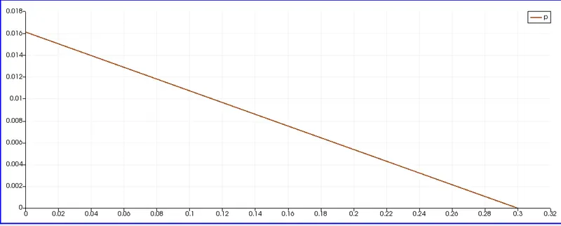
Pressure drop between pipe section from 1.3m to 1.6m (fully developed region) ,
Maximum wall shear stress ,
From pressure drop graph , `DeltaP = 0.016111 - 0 = 0.016111 m^2/s^2`
This is kinematic pressure , to convert it to dynamic pressure we have to multiply with density.
`DeltaP = 0.016111 "*" 997 = 16.062667 (Kg)/(ms^2)`
All other values we get directly from the plot. These values are compared to the analytical values in the below table,
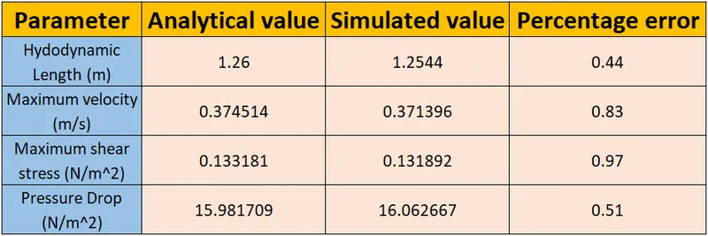
Here we can see that the error is very small and hence the simulation is accurate representation.
CONCLUSION
An axi-symmetric flow by applying the wedge boundary condition using OpenFOAM software has been simulated successfully and the results has been validated using Hagen- Poiseuille's equations.