Week 8 - Simulation of a backward facing step in OpenFOAM

AIM

To simulate an incompressible-laminar-viscous flow through the backward facing step geometry using OpenFOAM. Transient simulation should be performed.

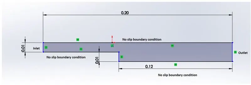
The mesh specification should be as follows,

1. Number of cells along the x direction (longer dimension) = 200
2. Number of cells along the longer y direction = 20;

The domain specifications are provided in the following figure,

THEORY

An OpenFOAM is an open source software for Computational Fluid Dynamics. It is used to find solutions for CFD problems by pre-processing and post-processing the problem. The full form of OpenFOAM is Open source Field Operation And Manipulation.

The procedure to solve a CFD problem using OpenFOAM is as follows,

1. Case Setup:- In this step the input data files are given , this includes things like start time , end time , time step etc…
2. Meshing:- In this step the mesh structure is created and the boundary conditions are specified.
3. Solver:- It is used to solve the governing equations of the fluid flow as per the given conditions.
4. Post-Processing:- This step helps in visualizing the solutions that have been solved.

OBJECTIVE

1. To perform two case studies given below and compare the results ,

Case 1 - Simulate the flow without using any grading factor (i.e., GF = 1)

Case 2 - Simulate the flow with grading factor of 0.2. The cells should be finer near the walls (includig the step wall).

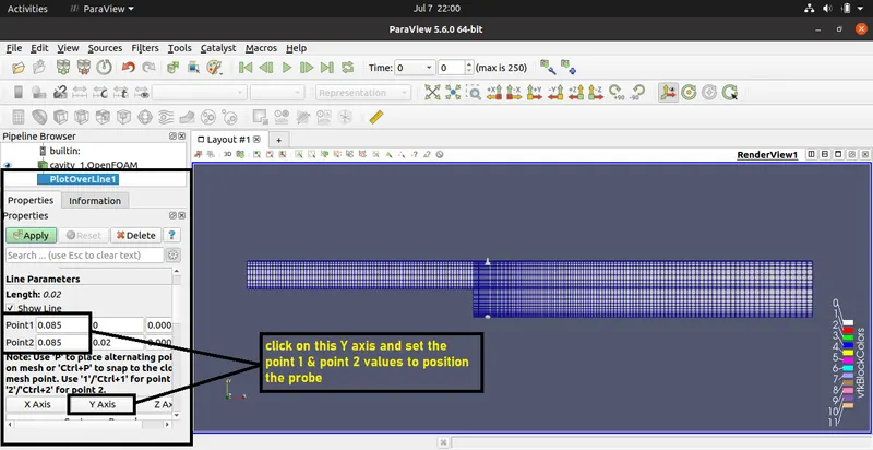
2. To measure the velocity profile at 0.085 m from the inlet of the geometry for both case studies and compare.

PROCEDURE

1) Pre-processing

• Obtain the reference case file from the OpenFOAM tutorials. In this case we need incompressible and laminar flow. Also the solver has to be transient. The corresponding solver is “icoFoam” , which is a transient solver for incompressible, laminar flow of Newtonian fluids. Inside this icoFoam directory we have our required geometry named “cavity”.
• After locating the required reference case file copy it to the OpenFOAM Run folder. This is done so as to prevent changing the source file. The code used to copy is “ cp -r folder name/ $FOAM_RUN/new folder name” . Here ‘folder name’ is the name of the folder to be copied and ‘new folder name’ is the new name given to that copied folder.
• Now we will go to the Run directory by using the code “cd $FOAM_RUN” , this will change the directory to Run.
• Inside the Run directory we have our copied folder. Now we will open that folder , inside which we will have the sub-folders containing initial condition , mesh and time values.

2) Mesh generation

• Now we will open the sub-folder “system” inside which we have ‘blockMeshDict’ file. This file contains the geometry and meshing data and it is opened using text editor to edit. This file after editing as per our requirement , which is to create backward facing step geometry is given below,

convertToMeters 0.001;

vertices
(
    (0 10 0)
    (80 10 0)
    (80 15 0)
    (0 15 0)
    (80 20 0)
    (0 20 0)
    (200 20 0)
    (200 15 0)
    (200 10 0)
    (200 0 0)
    (80 0 0)
    (0 10 1)
    (80 10 1)
    (80 15 1)
    (0 15 1)
    (80 20 1)
    (0 20 1)
    (200 20 1)
    (200 15 1)
    (200 10 1)
    (200 0 1)
    (80 0 1)   
    
);

blocks
(
    hex (0 1 2 3 11 12 13 14) (80 5 1) simpleGrading (1 5 1)
    hex (3 2 4 5 14 13 15 16) (80 5 1) simpleGrading (1 0.2 1)
    hex (2 7 6 4 13 18 17 15) (120 5 1) simpleGrading (5 0.2 1)
    hex (1 8 7 2 12 19 18 13) (120 5 1) simpleGrading (5 5 1)
    hex (10 9 8 1 21 20 19 12) (120 10 1) simpleGrading (5 5 1)
);

edges
(
);

boundary
(
    inlet
    {
        type patch;
        faces
        (
            (0 11 14 3)
            (3 14 16 5)
        );
    }
    outlet
    {
        type patch;
        faces
        (
            (6 17 18 7)
            (7 18 19 8)
            (8 19 20 9)
        );
    }
    frontAndBack
    {
        type empty;
        faces
        (
            (2 1 0 3)
            (4 2 3 5)
            (6 7 2 4)
            (7 8 1 2)
            (8 9 10 1)
            (15 13 18 17)
            (13 12 19 18)
            (12 21 20 19)
            (16 14 13 15)
            (14 11 12 13)
        );
    }
    noSlipWalls
    {
     	type wall;
     	faces
     	(
     	    (4 5 16 15)
     	    (6 4 15 17)
     	    (1 10 21 12)
     	    (1 12 11 0)
     	    (9 20 21 10)
        );
    }	
);

mergePatchPairs
(
);

• This given code is for Case 2.
• First the conversion to meter is defined. Here we have used values in millimeters for specifying coordinates in the 3-D Cartesian coordinate systemand hence the converting that to meters means multiplying by 0.001 .
• Then we specify the vertices coordinate values as per the given dimensions of the geometry.
• After that we define the blocks. We have split the given geometry into 5 blocks as shown below,

Blocks are defined by specifying the ordered list of vertex labels and the mesh size of that block. The vertex list should contain 8 vertices. Grading values are also specified here.

Grading

Grading will specify the grid size variation from start to end grid in the direction of the axis in which the grading is done.It is an essential part of meshing because the accuracy of a CFD solution is governed by the number of cells in the grid. So in the areas of the geometry where large variations occur from point to point it is better to have finer mesh and at areas with relatively less variation we can have coarser mesh.

Grading is specified by cell expansion ratio value.

`"Cell expansion ratio" = ("width of the end cell")/("width of the start cell")`

For Case 1 we will write, simpleGrading(1 1 1) for all 5 blocks, meaning that the value of cell expansion ratio in x,y & z direction is equal to 1. This will create a grid which is equally spaced throughout the geometry.

For Case 2 the values of grading is different for the 5 blocks. To better understand let us look at grading done for block 3.

For block 3 we need to have finer grids near to the walls. So we have wrote the code as simpleGrading (5 0.2 1). This means that along x-axis the expansion ratio is 5 and will create grids with start cell width equal to `(1/5)^(th)` of the end cell width. So this will give us finer grid at the walls along x-axis.

Now along y-axis we have given the expansion ratio value as 0.2 . This means that the end cell width is equal to `(1/5)^(th)` of the start cell width. Giving us finer grid at the walls along the y-axis.

Similarly we will do the grading for other 4 blocks.

• Next we will define the boundary patches. Here the patches basically represents each region in the geometry which will be named as per our convenience.

For example in our case we have defined the first patch as inlet , inside we will specify the vertices of those faces at the inlet. The order in which the vertices are specified must be such that , looking from inside the block and starting with any vertex, the face must be traversed in a clockwise direction to define the other vertices.

• Now to generate the mesh we will save this code. After that we will generate this mesh by running “blockMesh” command on this “blockMeshDict” file.

3) Boundary and initial conditons

• Now we will open the other sub-folder named “0”. This folder contains the boundary and initial conditions for pressure (p) and velocity (U).
• We will modify these conditions as per our requirement.
• The edited boundary and initial conditions of pressure is shown below,

dimensions      [0 2 -2 0 0 0 0];

internalField   uniform 0;

boundaryField
{
    inlet
    {
        type            zeroGradient;
       
    }

    outlet
    {
        type            fixedValue;
        value           uniform 0;
    }

    frontAndBack
    {
        type            empty;
    }
    
    noSlipWalls
    {
    	type 	        zeroGradient;
    }
}

At the outlet we have considered that the gauge pressure to be 0 , i.e 1 atm.

• The edited boundary and initial conditions of velocity is shown below,

  dimensions      [0 1 -1 0 0 0 0];
  
  internalField   uniform (0 0 0);
  
  boundaryField
  {
      inlet
      {
          type            fixedValue;
          value           uniform (1 0 0);
      }
  
      outlet
      {
          type            zeroGradient;
      }
  
      frontAndBack
      {
          type            empty;
      }
      
      noSlipWalls
      {
      	type 	        noSlip;
      }
  }
  ​

• At the inlet we have specified the velocity to be uniform 1m/s.

4) Control values

• In the system sub folder we have a file named “controlDict” , this contains the values like start time , time step , end time etc… for simulation. The code for this is shown below,

  application     icoFoam;
  
  startFrom       startTime;
  
  startTime       0;
  
  stopAt          endTime;
  
  endTime         0.5;
  
  deltaT          0.0001;
  
  writeControl    timeStep;
  
  writeInterval   20;
  
  purgeWrite      0;
  
  writeFormat     ascii;
  
  writePrecision  6;
  
  writeCompression off;
  
  timeFormat      general;
  
  timePrecision   6;
  
  runTimeModifiable true;​

  In this code we have changed the time step value to 0.0001, so as to satisfy the CFL condition.

Solver

Now to solve the governing equations we run the command “icoFoam” , which is the solver used.

Post-processing

To visualize the solved geometry and the simulation we will run the command “paraFoam” . This is a post-processing tool supplied with OpenFOAM. This will open the paraview tool window shown below,

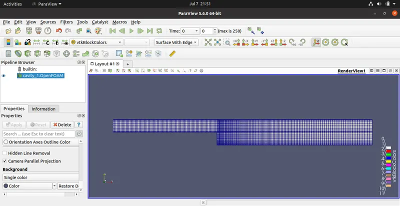
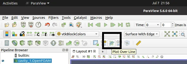
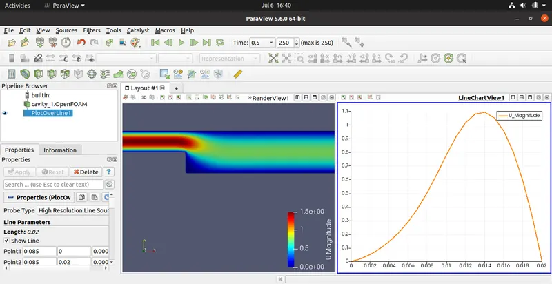
Now to measure the velocity profile at 0.085 m from the inlet of the geometry , we will use plot over line tool in paraview. This tool is shown below,

Now inside the properties of this tool change the values as shown below,

RESULTS

Let us look at the results for Case 1 ,

The mesh and the geometry is shown below,

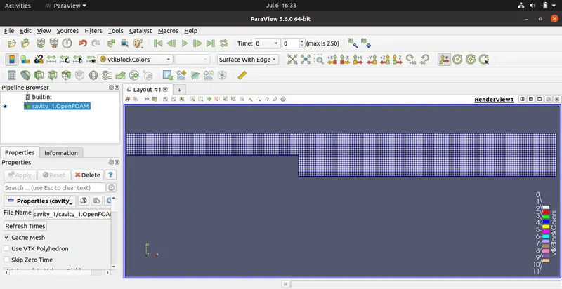
Here we can see that the size of the mesh is same at all areas.

The flow at the end of the simulation is shown below ,

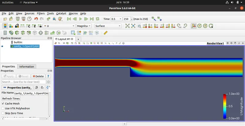
The flow gets expanded after the backward facing step and the velocity drops significantly.

The velocity profile at 0.085m is shown below,

Now let us look at the results for Case 2 ,

The mesh and the geometry is shown below,

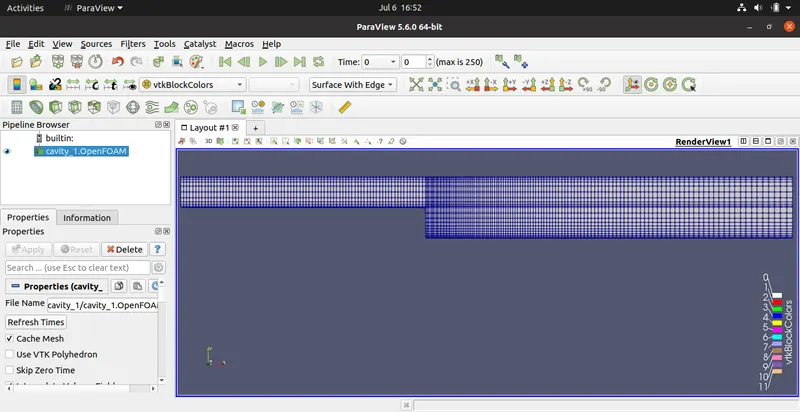
Here we can see that the size of the mesh is finer near to the walls.

The flow at the end of the simulation is shown below ,

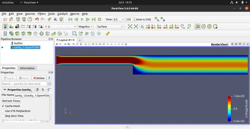
The flow gets expanded after the backward facing step and the velocity drops significantly.

The velocity profile at 0.085m is shown below,

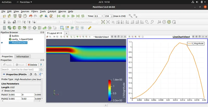
On comparing the velocity profiles for the two cases we can find that the maximum velocity value is different. For Case 1 the maximum velocity is 1.093 where as in case of Case 2 maximum velocity is 1.083. This shows us that we get much more accurate results if we use finer mesh.

CONCLUSION

Transient simulation of an incompressible-laminar-viscous flow through the backward facing step geometry using OpenFOAM has been done successfully.