Week 5.1 - Mid term project - Solving the steady and unsteady 2D heat conduction problem

Aim

1. To simulate the steady state 2D heat equation using iterative solvers

2. To simulate the transient 2D heat equation using implicit and explicit schemes

Solution

Heat equation - Theory

The general 3D heat equation can be written as

`(delu)/(delt) + alpha((∂^2 T )/(∂ x^2) + (∂^2 T)/(∂ y^2) + (∂^2 T)/(∂ x^2)) = 0`

The first term is the time derivative term, the second term is the spatial derivative, and alpha is the thermal diffusivity of the medium.

Steady state 2D heat equation

The equation in 2D can be written in steady state, as follows

`(∂^2 T)/(∂x^2 )+(∂^2 T)/(∂y^2 )=0`

The time derivative term is zero, since the rate of change of temperature with time is zero.

The equation can be discretized by central differencing as follows

WRT X

`(∂^2T)/( ∂x^2) = (T (i − 1 , j) − 2 T( i , j) + T (i + 1 , j ))/(Δ x ^2)`

WRT Y

`(∂^2T)/( ∂y^2) = (T (i , j-1) − 2 T( i , j) + T (i , j+1 ))/(Δ y ^2)`

Since we have assumed nx = ny, `Δ x ^2=Δy ^2`

Therefore, the equation is

`T (i,j) = 1 /4 ( T( i − 1 , j )+ T (i + 1 , j )+ T (i , j − 1) + T (i , j + 1 )`

This equation is solved in Matlab using three iterative schemes - Jacobi, Gauss-Seidel and Successive Over Relaxation (SOR).

The matlab script is as follows.

% 2D heat conduction - Steady state 

clear all
close all
clc

% Inputs

nx = 10;
ny = 10;
x = linspace(0,1,nx);
y = linspace(0,1,ny);
dx = x(2) - x(1);
dy = y(2) - y(1);
[xx,yy] = meshgrid(x,y);

% Defining boundary conditions

T = ones(nx,ny);
T(1,:) = 900;
T(end,:) = 600;
T(:,1) = 400;
T(:,end) = 800;

Told = T;

% Errors 
error_tol = 1e-4;
start_error = 9e9;

k = 2*((dx^2 + dy^2)/(dx^2*dy^2));

%% SOLVERS

iter_solver = questdlg('Select iterative solver','Solver','Jacobi','Gauss-Seidel','SOR','Jacobi');

switch iter_solver
    case 'Jacobi'
        ITSR = 1;
    case 'Gauss-Seidel'
        ITSR = 2;
    case 'SOR'
        ITSR = 3;
end 

if ITSR == 1
    tic;
    T_jacobi = ss_jacobi(start_error,error_tol,xx,yy,nx,ny,dx,dy,T,k,Told);
    Time_jacobi = toc;
    
elseif ITSR == 2
   tic;
    T_gauss = ss_gauss(start_error,error_tol,xx,yy,nx,ny,dx,dy,T,k,Told);
    Time_gauss = toc;
    
elseif ITSR == 3
    tic;
    T_sor = ss_sor(start_error,error_tol,xx,yy,nx,ny,dx,dy,T,k,Told);
    Time_sor = toc;
end

The functions can be found below.

1. Jacobi

function T = ss_jacobi(start_error,error_tol,xx,yy,nx,ny,dx,dy,T,k,Told)

jacobi_iter = 1;
while(start_error > error_tol)
    for i = 2:nx-1
        for j = 2:ny-1
            term1 = (Told(i-1,j) + Told(i+1,j))/(k*dx^2);
            term2 = (Told(i,j-1) + Told(i,j+1))/(k*dy^2);
            T(i,j) = term1 + term2;
        end
    end
    
    start_error = max(max(abs(Told-T)));
    Told = T;
    jacobi_iter = jacobi_iter + 1;
    
    figure(1)
    
    [c,d] = contourf(xx,yy,T);
    colormap(jet);
    colorbar;
    title('Number of Jacobi iterations (IMPLICIT):',jacobi_iter);
    xlabel('X-axis');
    ylabel('Y-axis');
    clabel(c,d);
    %pause(0.03)
end
fprintf('Number of Jacobi iterations: %d',jacobi_iter);
end

2. Gauss-Seidel

function T = ss_gauss(start_error,error_tol,xx,yy,nx,ny,dx,dy,T,k,Told)

gauss_iter = 1;
while(start_error > error_tol)
    for i = 2:nx-1
        for j = 2:ny-1
            
            T(i,j) = (((T(i-1,j) + Told(i+1,j))/dx^2)+((T(i,j-1)+Told(i,j+1))/dy^2))/k;
        end
    end
    
    start_error = max(max(abs(Told-T)));
    Told = T;
    gauss_iter = gauss_iter + 1;
    
    figure(2)
    
    [c,d] = contourf(xx,yy,T);
    colormap(jet);
    colorbar;
    title('Number of Gauss iterations (IMPLICIT):',gauss_iter);
    xlabel('X-axis');
    ylabel('Y-axis');
    clabel(c,d);
    %pause(0.03)
end
fprintf('Number of Gauss iterations:',gauss_iter);
end

3. SOR

function T = ss_sor(start_error,error_tol,xx,yy,nx,ny,dx,dy,T,k,Told)

sor_iter = 1;
omega = 1.7;

while(start_error > error_tol)
    for i = 2:nx-1
        for j = 2:ny-1
            
            T_gs = (((T(i-1,j) + Told(i+1,j))/dx^2)+((T(i,j-1)+Told(i,j+1))/dy^2))/k;
            T(i,j) = omega*T_gs + (1-omega)*(Told(i,j));
        end
    end
    
    start_error = max(max(abs(Told-T)));
    Told = T;
    sor_iter = sor_iter + 1;
    
    figure(3)
    
    [c,d] = contourf(xx,yy,T);
    colormap(jet);
    colorbar;
    title('Number of SOR iterations (IMPLICIT):',sor_iter);
    xlabel('X-axis');
    ylabel('Y-axis');
    clabel(c,d);
    %pause(0.03)
end
fprintf('Number of SOR iterations:',sor_iter);
end

Results

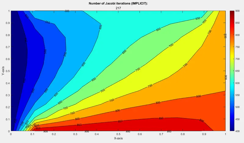
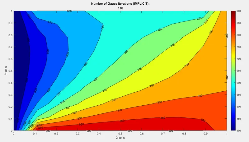
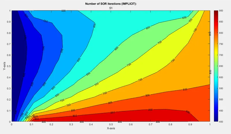
Steady state - Implicit schemes

1. Jacobi

2. Gauss-Seidel

3. SOR

Transient 2D heat equation - (Unsteady)

The general 2D equation is

`α ((∂ ^2 T)/( ∂ x ^2) +( ∂^ 2 T)/( ∂ y ^2) )= (∂ T)/( ∂ t)`

The equation can be discretized by central differencing and the time derivative part by forward differencing

WRT X

`(∂ ^2 T)/( ∂ x^ 2) = (T( i − 1 , j )− 2 T (i , j) + T( i + 1 , j))/ (Δ x^ 2)`

WRT Y

`(∂^2T)/( ∂y^2) = (T (i , j-1) − 2 T( i , j) + T (i , j+1 ))/(Δ y ^2)`

WRT time gradient

`(∂ T)/( ∂ t) = (T^( n + 1)( i , j )− T n ( i , j ))/(Δ t)`

Constants k1 and k2 can be defined, where

`k1=α(Δt)/(Δx^2)`

`k2=α(Δt)/(Δy^2)`

Since we have assumed nx = ny, `Δ x ^2=Δy ^2`

The equation becomes`T ^(n + 1 )( i , j )= (T^ n ( i , j) + k1 ( T (i − 1 , j) + T (i + 1 , j )) ^(n+1)+ k2 ( T (i , j − 1) + T (i , j + 1 ))^(n + 1))/( 1 + 2 K 1 + 2 K 2)`

The transient equation can be solved using both explicit and implicit schemes

1. Explicit scheme

The matlab script for solving the transient equation using explicit scheme is as follows

% 2D heat conduction - unsteady (transient)

clear all
close all
clc

% Input parameters
%Grid points
nx = 40;
ny = nx;
nt = 140000;

x = linspace(0,1,nx);
y = linspace(0,1,ny);

dx = x(2) - x(1);
dy = y(2) - y(1);
dt = 0.01;

alpha = 1.88e-5;

[xx,yy] = meshgrid(x,y);

% Boundary conditions
T = ones(nx,ny);
T(1,:) = 900;
T(end,:) = 600;
T(:,1) = 400;
T(:,end) = 800;

Told = T;

% Rounding off corner values - Average
T(1,1) = (400+900)/2;
T(1,ny) = (900+800)/2;
T(nx,1) = (400+600)/2;
T(nx,ny) = (600+800)/2;

% Errors 
error_tol = 1e-4;
start_error = 9e9;

k1 = alpha*(dt/dx^2);
k2 = alpha*(dt/dy^2);

%% Solver

iter_solver = 1;

tic;
if iter_solver == 1
    unsteady_explicit = 1;
    for k = 1:nt
        start_error = 9e9;
        while(start_error > error_tol)
            for i = 2:nx-1
                for j = 2:ny-1
                    term1 = Told(i,j);
                    term2 = k1*(Told(i+1,j) - 2*Told(i,j) + Told(i-1,j));
                    term3 = k2*(Told(i,j+1) - 2*Told(i,j) + Told(i,j-1));
                    T(i,j) = term1+term2+term3;
                end
            end
            start_error = max(max(abs(Told - T)));
            Told = T;
            unsteady_explicit = unsteady_explicit + 1;
        end
        
    end
end

figure(1)
    
    [c,d] = contourf(xx,yy,T);
    colormap(jet);
    colorbar;
    title('Number of  iterations (UNSTEADY EXPLICIT):',unsteady_explicit);
    xlabel('X-axis');
    ylabel('Y-axis');
    clabel(c,d);
    %pause(0.03)

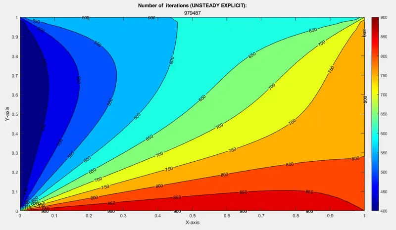
Results

Unsteady (transient) - Explicit

1. Implicit schemes

This equation is solved in Matlab using three iterative schemes - Jacobi, Gauss-Seidel and Successive Over Relaxation (SOR).

The matlab script is as follows.

% 2D heat conduction - unsteady (transient)

clear all
close all
clc

% Input parameters
%Grid points
nx = 40;
ny = nx;
nt = 140000;

x = linspace(0,1,nx);
y = linspace(0,1,ny);

dx = x(2) - x(1);
dy = y(2) - y(1);
dt = 1e-2;

alpha = 1.88e-5;

[xx,yy] = meshgrid(x,y);

% Boundary conditions
T = 298*ones(nx,ny);
T(1,:) = 900;
T(end,:) = 600;
T(:,1) = 400;
T(:,end) = 800;

% Rounding off corner values - Average
T(1,1) = (400+900)/2;
T(1,ny) = (900+800)/2;
T(nx,1) = (400+600)/2;
T(nx,ny) = (600+800)/2;

Told = T;
Tprev = Told;

% Errors 
error_tol = 1e-4;
start_error = 9e9;

k1 = alpha*(dt/(dx^2));
k2 = alpha*(dt/(dy^2));

omega = 2/(1+sin(pi*dx));
CFL = alpha*(dt/(dx^2));

%% SOLVERS

iter_solver = questdlg('Select iterative solver','Solver','Jacobi','Gauss-Seidel','SOR','Jacobi');

switch iter_solver
    case 'Jacobi'
        ITSR = 1;
    case 'Gauss-Seidel'
        ITSR = 2;
    case 'SOR'
        ITSR = 3;
end 

if ITSR == 1
    tic;
    T_jacobi = unst_jacobi(start_error,error_tol,xx,yy,nx,ny,nt,dx,dy,T,k1,k2,Told,Tprev);
    Time_jacobi = toc;
    
elseif ITSR == 2
   tic;
    T_gauss = unst_gauss(start_error,error_tol,xx,yy,nx,ny,nt,dx,dy,T,k1,k2,Told,Tprev);
    Time_gauss = toc;
    
elseif ITSR == 3
    tic;
    T_sor = unst_sor(start_error,omega,error_tol,xx,yy,nx,ny,nt,dx,dy,T,k1,k2,Told,Tprev);
    Time_sor = toc;
end

The functions can be found below.

1. Jacobi

function T = unst_jacobi(start_error,error_tol,xx,yy,nx,ny,nt,dx,dy,T,k1,k2,Told,Tprev)

jacobi_iter = 1;
for k = 1:nt
   start_error = 9e9;
while(start_error > error_tol)
    for i = 2:nx-1
        for j = 2:ny-1
             term1 = (1+(2*k1)+(2*k2))^(-1);
             term2 = k1*term1;
             term3 = k2*term1;
             H = (Told(i-1,j)+ Told(i+1,j));
             V = (Told(i,j-1) + Told(i,j+1));
             T(i,j) = (Tprev(i,j)*term1)+ term2*H + term3*V;
        end
    end
    
    start_error = max(max(abs(Told-T)));
    Told = T;
    jacobi_iter = jacobi_iter + 1;
    
end
    Tprev = T;
    
    
end
figure(1)
    
    [c,d] = contourf(xx,yy,T);
    colormap(jet);
    colorbar;
    title('Number of Jacobi iterations (UNSTEADY IMPLICIT):',jacobi_iter);
    xlabel('X-axis');
    ylabel('Y-axis');
    clabel(c,d);
    %pause(0.03)
    fprintf('Number of Jacobi iterations: %d',jacobi_iter);
    
end

2. Gauss-Seidel

function T = unst_gauss(start_error,error_tol,xx,yy,nx,ny,nt,dx,dy,T,k1,k2,Told,Tprev)

gauss_iter = 1;
for k = 1:nt
   start_error = 9e9;
while(start_error > error_tol)
    for i = 2:nx-1
        for j = 2:ny-1
             term1 = (1+(2*k1)+(2*k2))^(-1);
             term2 = k1*term1;
             term3 = k2*term1;
             H = (T(i-1,j)+ T(i+1,j));
             V = (T(i,j-1) + T(i,j+1));
             T(i,j) = (Tprev(i,j)*term1)+term2*H+term3*V;
        end
    end
    
    start_error = max(max(abs(Told-T)));
    Told = T;
    gauss_iter = gauss_iter + 1;
    
end
    Tprev = T;
end
figure(1)
    
    [c,d] = contourf(xx,yy,T);
    colormap(jet);
    colorbar;
    title('Number of Gauss iterations (UNSTEADY IMPLICIT):',gauss_iter);
    xlabel('X-axis');
    ylabel('Y-axis');
    clabel(c,d);
    %pause(0.03)
    fprintf('Number of Gauss iterations: %d',gauss_iter);
end

3. SOR

function T = unst_sor(start_error,omega,error_tol,xx,yy,nx,ny,nt,dx,dy,T,k1,k2,Told,Tprev)


sor_iter = 1;
for k = 1:nt
   start_error = 9e9;
while(start_error > error_tol)
    for i = 2:nx-1
        for j = 2:ny-1
             term1 = (1+(2*k1)+(2*k2))^(-1);
             term2 = k1*term1;
             term3 = k2*term1;
             H = (T(i-1,j)+ Told(i+1,j));
             V = (T(i,j-1) + Told(i,j+1));
             T(i,j) = (Tprev(i,j)*term1)+term2*H+term3*V;
             T(i,j) = ((1-omega)*Tprev(i,j))+(omega*T(i,j));
        end
    end
    
    start_error = max(max(abs(Told-T)));
    Told = T;
    sor_iter = sor_iter + 1;
    
end
    Tprev = T;
end
figure(1)
    
    [c,d] = contourf(xx,yy,T);
    colormap(jet);
    colorbar;
    title('Number of SOR iterations (UNSTEADY IMPLICIT):',sor_iter);
    xlabel('X-axis');
    ylabel('Y-axis');
    clabel(c,d);
    %pause(0.03)
    fprintf('Number of SOR iterations: %d',sor_iter);
end

Results

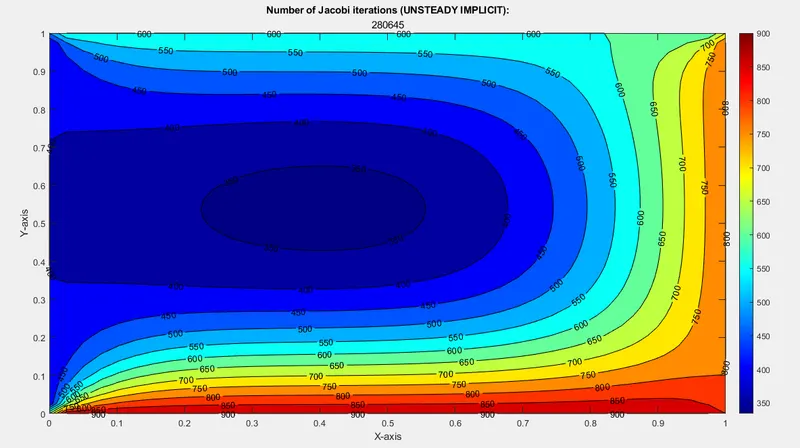
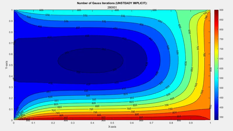
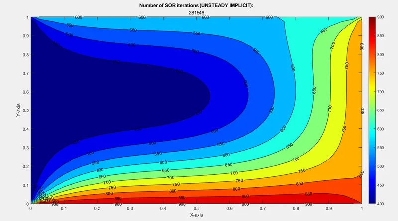
Unsteady (transient) - Implicit schemes

1. Jacobi

2. Gauss - Seidel

3. SOR

Observations and inferences

The summary of the number of iteration for each scheme for both cases can be found below.

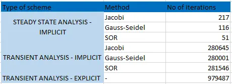
It can be clearly seen, that the SOR is the most time - efficient method for the steady state equation

The Jacobi method is slightly faster among the implicit methods, for solving the transient equation.

Conclusion

Thus, the 2D heat equation (steady state and transient) have been simulated using various (explicit and implicit) iteration schemes, and the results have been illustrated and compared.

The associated matlab m files have been attached below.