Week 3: Flow over a backward facing step
Objective
To simulate the flow over backward facing step with different mesh sizes and compare the results
Solution
The BFS stl file is imported into Converge and setup for simulation.
The dimensions of the geomtry are shown in the figure below
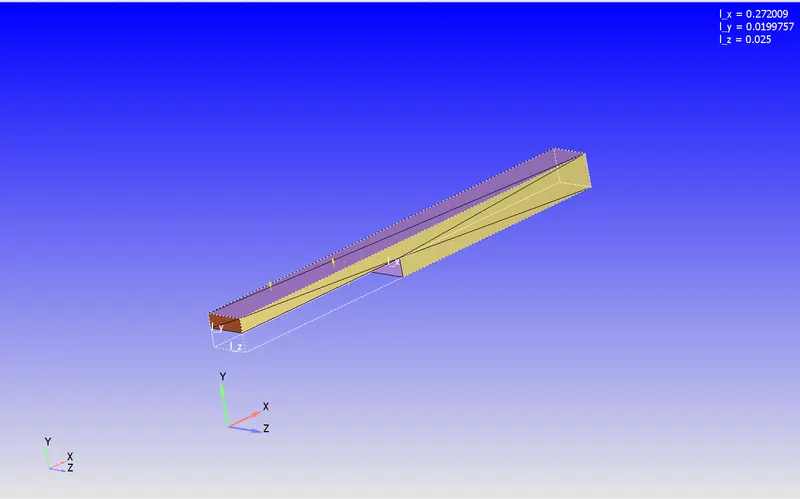
A time based simulation is selected with the material as Air.
The values for the global transport parameters and reaction mechanism are kept default.
Solver setup
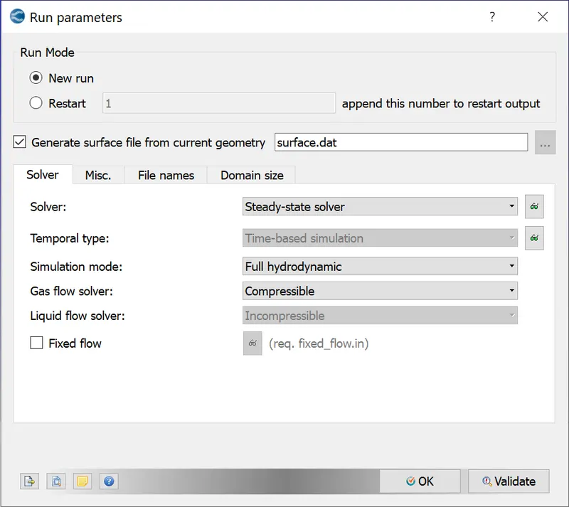
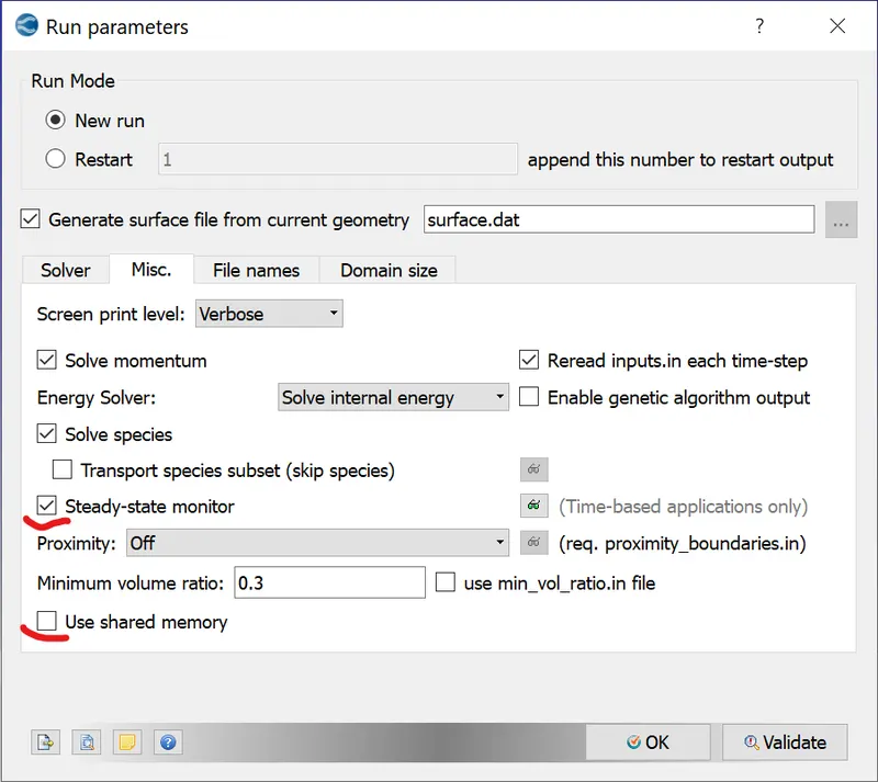
A steady state, full hydrodynamic compressible solver is selected as shown below. The steady state monitor is turned on, and the use of shared memory is unchecked
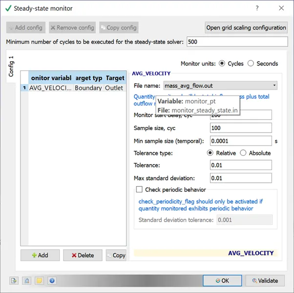
The steady state monitor can be defined as shown below
Simulation time parameters
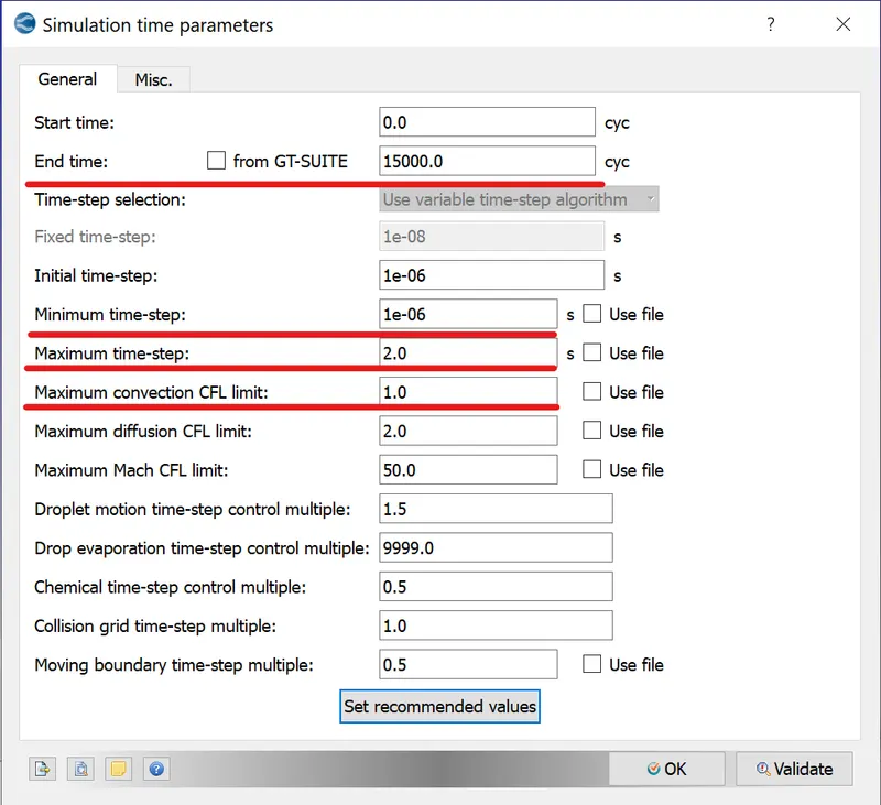
An end time of 15000 cycles is selected with minimum time step of 1e-6 s and max time step of 2.0 s. The convection CFL limit it set as 1.0. The values of the other parameters are maintained default.
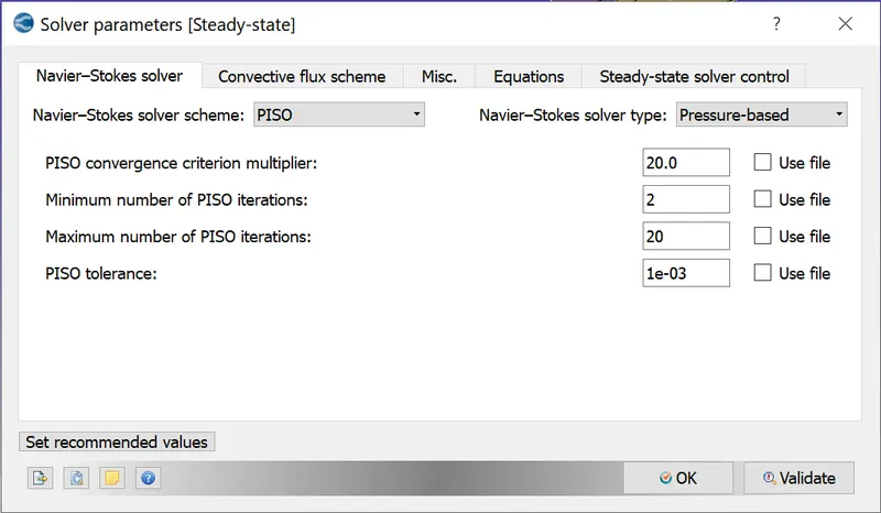
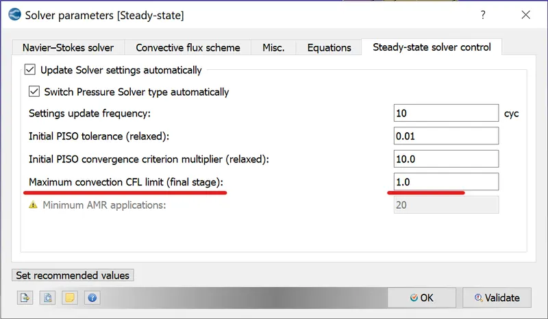
A Navier Stokes pressure based solver is selected, and under steady state solver control, the maximum CFL limit is given as 1.0 to reflect the value given under the simulation time parameters.
Boundary conditions and initialization
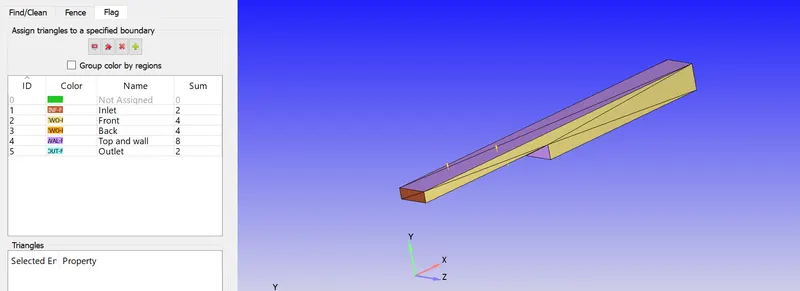
The sides of the geometry are flagged with the appropriate boundary, and assigned relevant boundary conditions.
Inlet
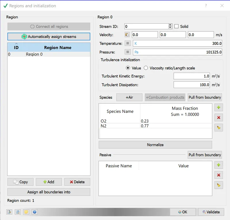
The pressure at the inlet is defined as 110325 Pa, with INFLOW boundary type and air as medium.
Outlet
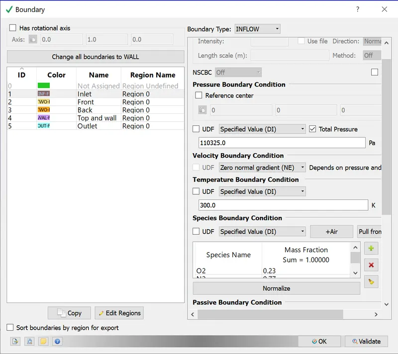
The pressure at the outlet is defined as 101325 Pa, with OUTFLOW boundary type and air as medium.
Top and walls
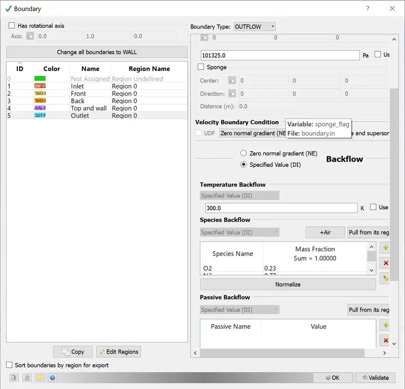
The top surface and walls are defined with law of wall and zero normal gradient for the TKE.
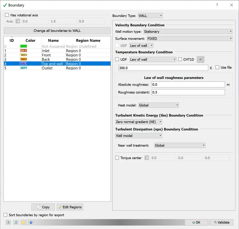
The front and back faces are defined as 2D walls.
Physical models
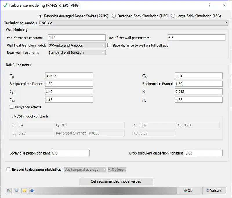
The RANS K-Epsilon model is selected as the turbulence model, with the values for the constants as shown below.
Grid size
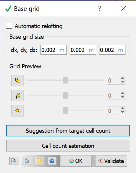
The base grid is defined with the required size along all three axes.
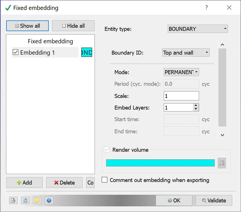
Fixed embedding at the boundaries of top and walls are added for further mesh refinement.
The output and post processing parameters are kept default, and the setup is completed for simulation.
The simulation is carried out using Cygwin, and the results are illustrated below.
Results
Grid size: dx - 2.0 e-3,dy - 2.0 e-3, dz - 2.0 e-3
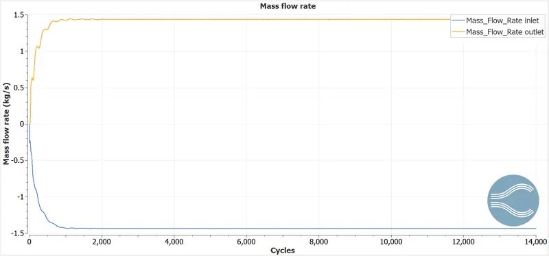
Mass flow rate
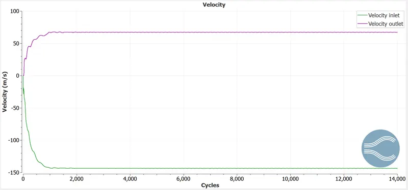
Velocity
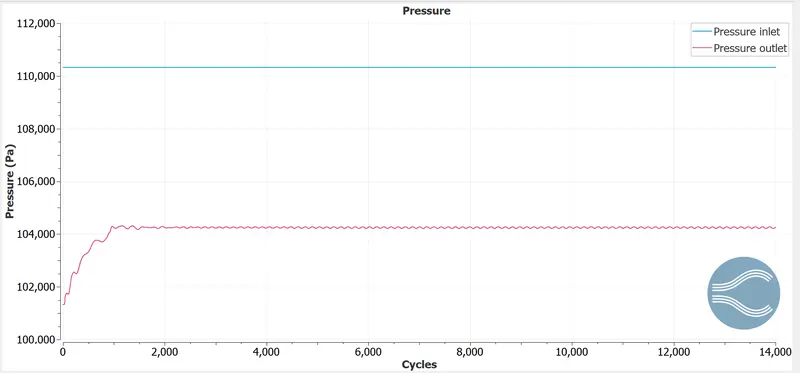
Pressure
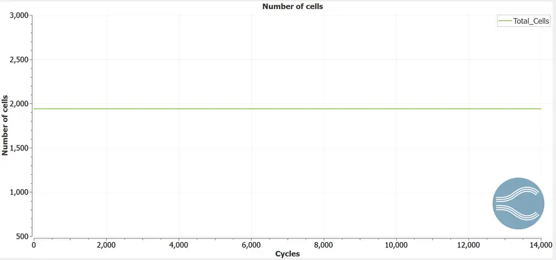
Number of cells
Paraview
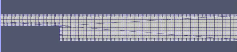
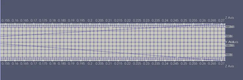
Mesh
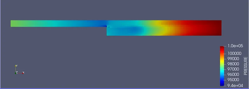
Pressure contour
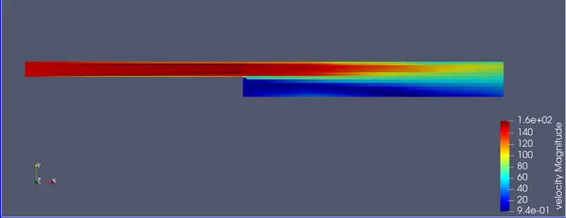
Velocity contour
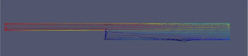
Glyph plot - Flow separation and recirculation
The vector field helps clearly visualize the flow separation occuring at the step. There is a recirculation zone at this region, which is at low pressure. The flow proceeds and reattaches at a further point along the tube, which is again a region of higher pressure.
Animation of pressure
Animation of velocity
Grid size: dx - 1.5 e-3,dy - 1.5 e-3, dz - 1.5e-3
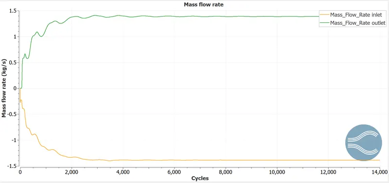
Mass flow rate
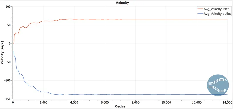
Velocity
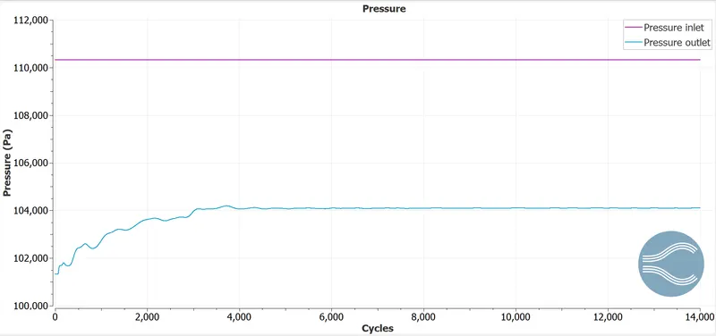
Pressure
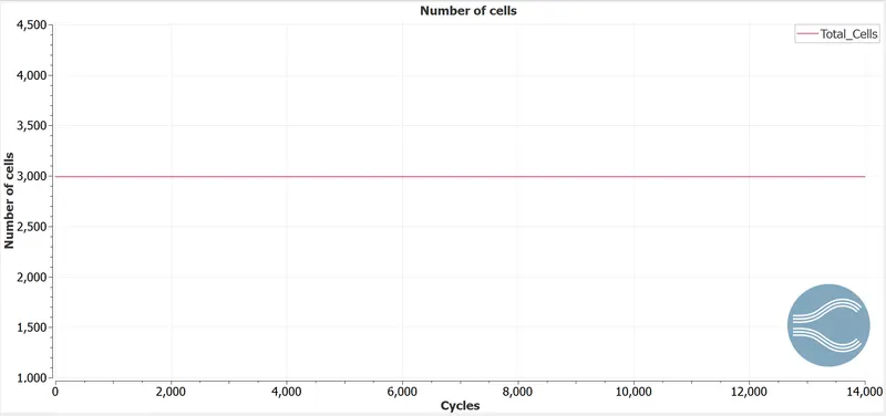
Number of cells
Paraview
Mesh
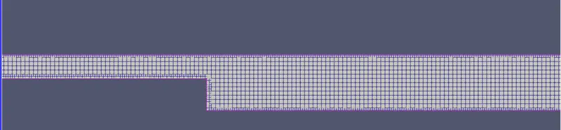
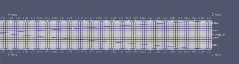
Pressure contour
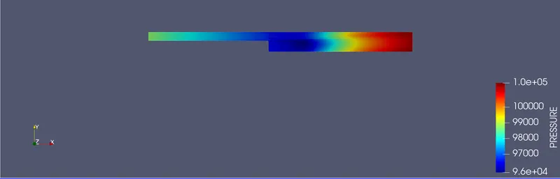
Velocity contour
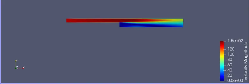
Glyph plot - Flow separation and recirculation
The vector field helps clearly visualize the flow separation occuring at the step. There is a recirculation zone at this region, which is at low pressure. The flow proceeds and reattaches at a further point along the tube, which is again a region of higher pressure.
Animation of pressure
Animation of velocity
Grid size: dx - 1.0 e-3,dy - 1.0 e-3, dz - 1.0 e-3
Mass flow rate
Velocity
Pressure
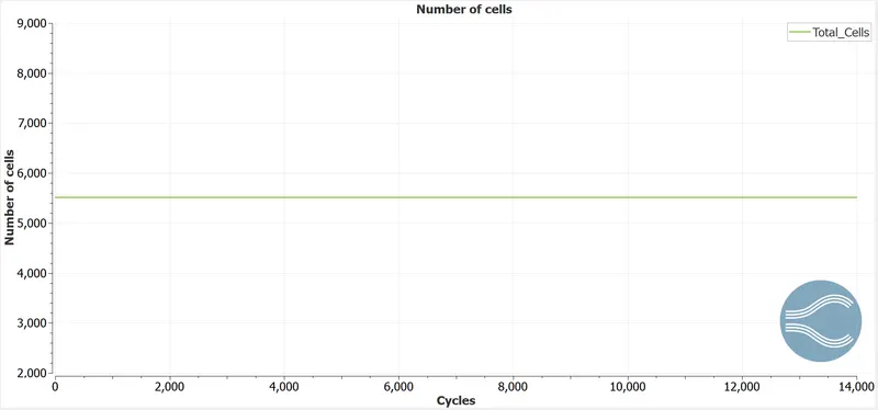
Number of cells
Paraview
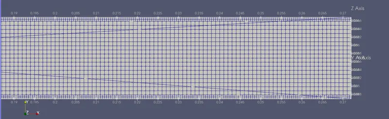
Mesh

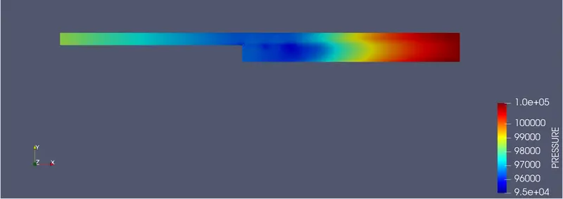
Pressure contour
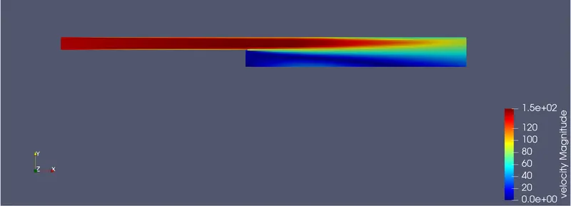
Velocity contour
Glyph plot - Flow separation and recirculation
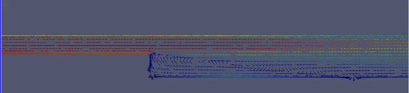
The vector field helps clearly visualize the flow separation occuring at the step. There is a recirculation zone at this region, which is at low pressure. The flow proceeds and reattaches at a further point along the tube, which is again a region of higher pressure.
Animation of pressure
Animation of velocity
Comparison
Mass flow rate
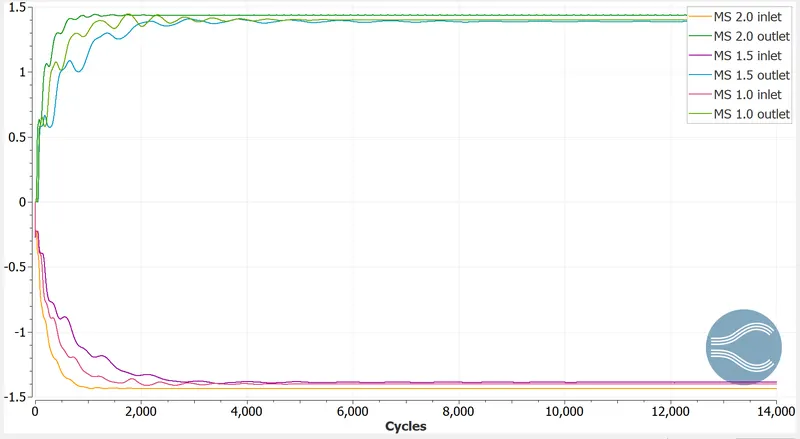
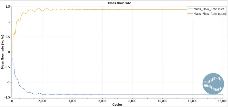
It can be seen from the plot above, that the peak mass flow rate is around 1.5 kg/s. The number of cycles needed to attain steady state reduces, as the mesh size increases.
Velocity
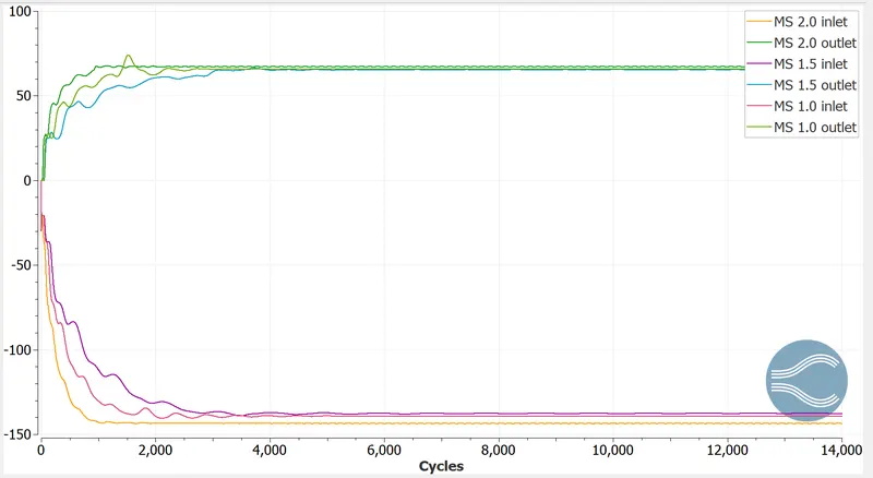
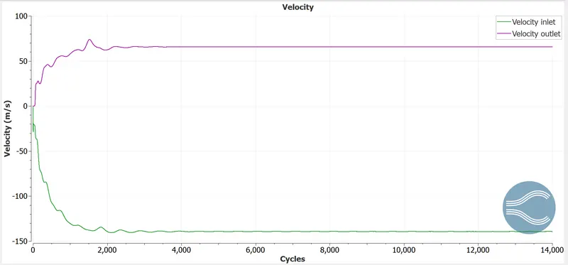
The peak velocity at the inlet is around 150 m/s and at the outlet is 75 m/s. This is due to the presence of high pressure at the outlet, compared to the inlet. The increase of mesh size helps steady state to be attained quicker.
Pressure
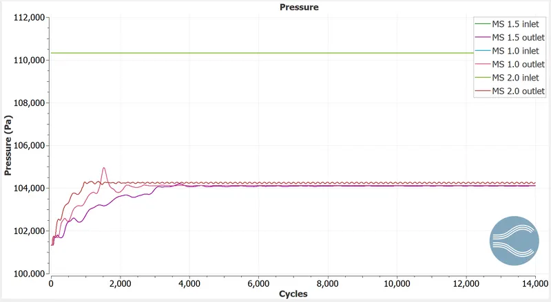
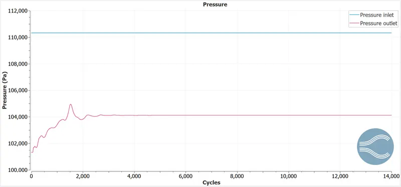
The pressure at the inlet is the same in all three cases. The pressure at the outlet converges faster to a steady state peak value of around 104,500 Pa in all three mesh sizes.
Number of cells
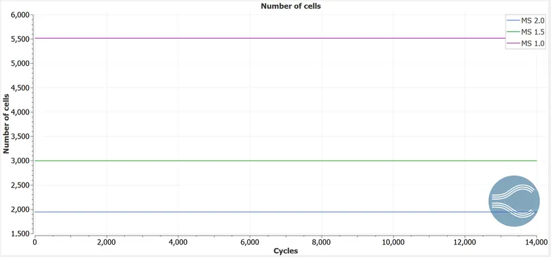
The number of cells increases at the mesh size increases, as highlighted in the image above. This increases the accuracy of computation at a slightly higher cost.
Conclusion
Thus the flow over a backward facing step is simulated for various mesh sizes and the results have been compared.