Week 4.2: Project - Transient simulation of flow over a throttle body
Objective
To perform the steady state simulation of flow over a throttle body and analyse the results.
Solution
The elbow stl file is imported into converge, and the geometry is scaled in order to convert units from mm to m.
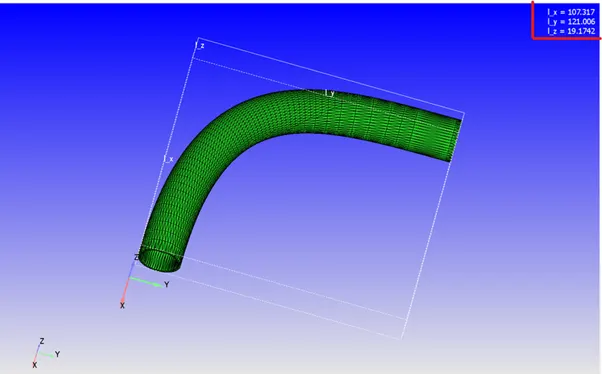
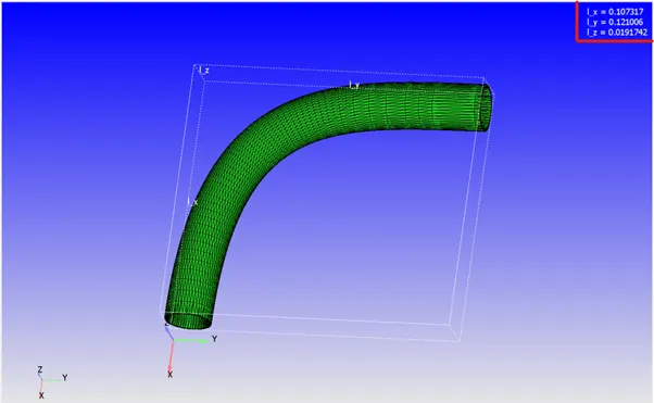
The geometry consists of a thickness, because of an outer and an inner surface. The outer surfaces of the geometry are removed using the boundary fence option
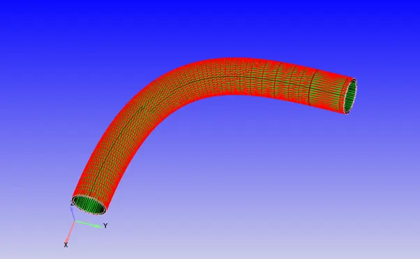
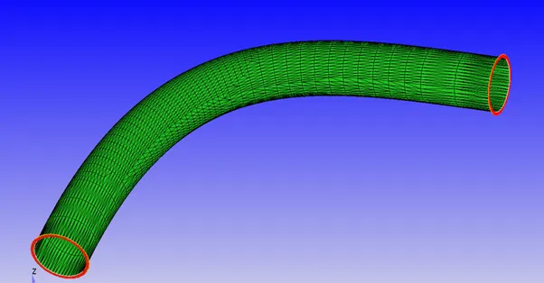
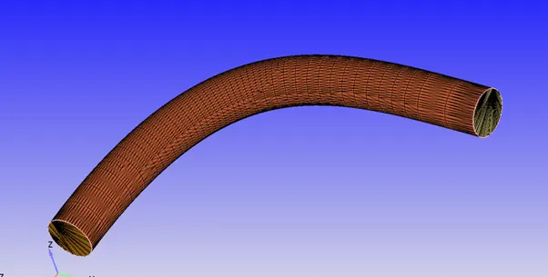
The final geometry ready for boundary flagging is shown below
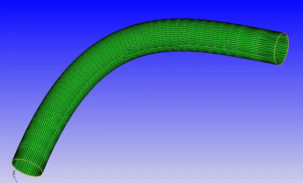
The two ends of the elbow are sealed using the Patch option, and the boundaries are flagged.
After using the diagnosis tool to ensure correctness of geometry, the case can be setup for simulation.
Case Setup
A time based simulation is selected with the material as Air.
The values for the global transport parameters and reaction mechanism are kept default.
Solver setup
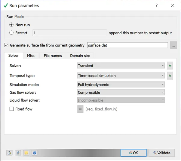
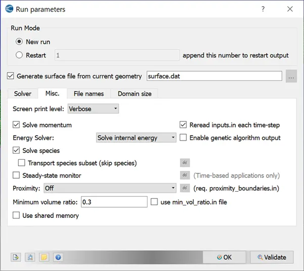
A transient, full hydrodynamic compressible solver is selected as shown below. The steady state monitor is turned off, and the use of shared memory is unchecked.
Simulation time parameters
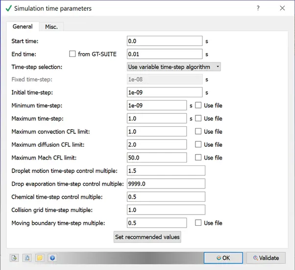
The end time can be calculated from the length of the pipe and the average velocity. From the steady state simulation, the average velocity at the inlet is around 190 m/s. For a length of pipe of 0.2m, the end time can be calculated as
End time = Length of pipe/velocity = 0.2/190 = 0.001 m.
For 10 passes of flow the end time is 10*0.001 = 0.01s.
The minimum time step is given as 1e-9s.
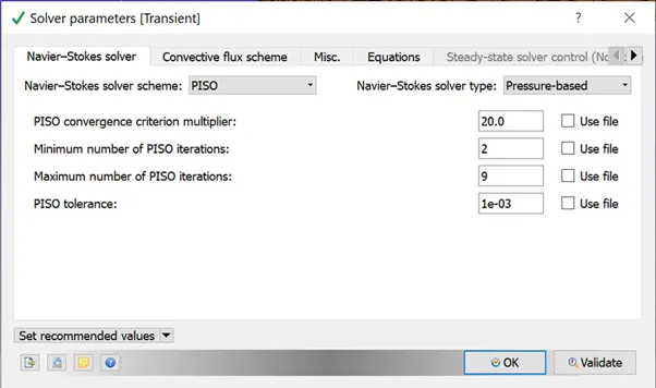
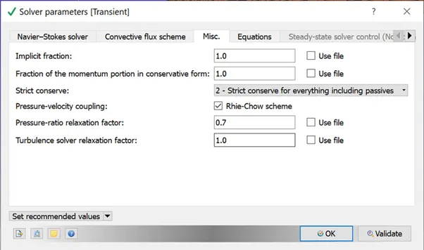
A Navier Stokes pressure based solver is selected, and strict conserve is set to 2, for conservation.
Boundary conditions and initialization
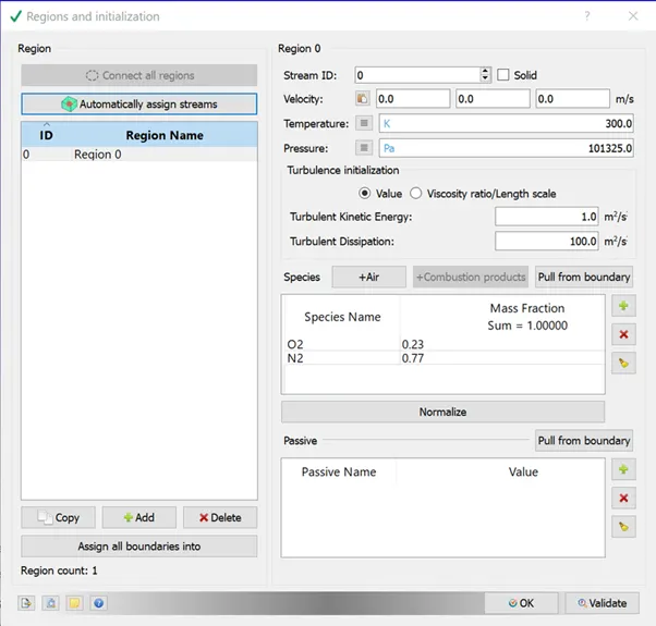
The sides of the geometry are flagged with the appropriate boundary, and assigned relevant boundary conditions.
Boundary flagging
The inlet, outlet and the elbow pipe surface are assigned separate boundaries.
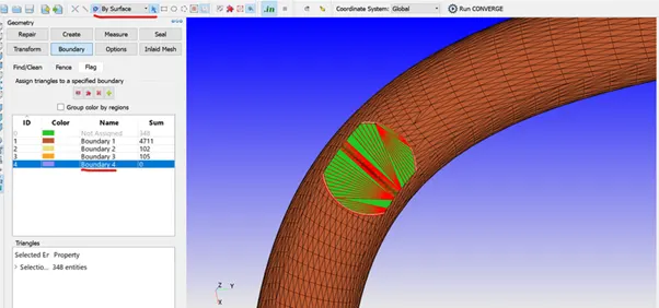
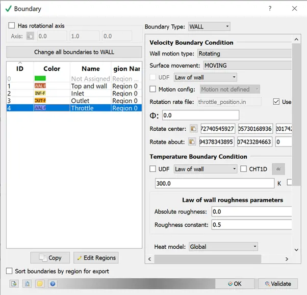
The throttle body is assigned to a boundary using the selection by surface option.
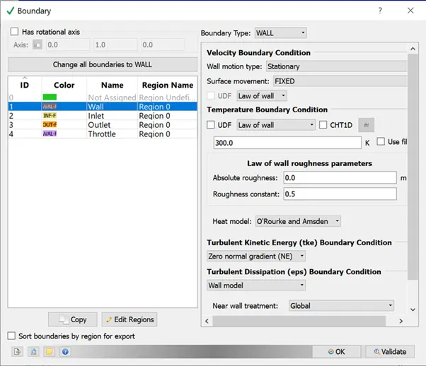
Wall
The walls are defined with law of wall and zero normal gradient for the TKE.
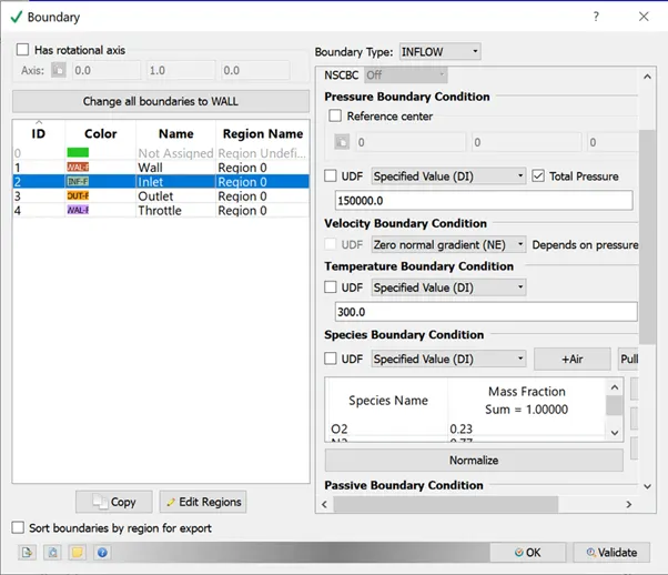
Inlet
The pressure at the inlet is defined as 1.5 e^5 bar, with INFLOW boundary type and air as medium.
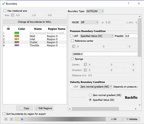
Outlet
The pressure at the outlet is defined as 1e^5 bar, with OUTFLOW boundary type and air as medium.
Throttle
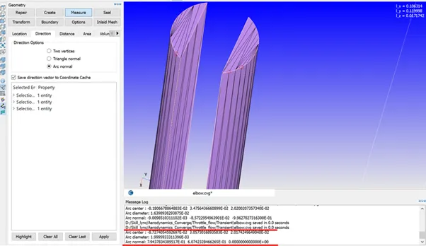
The throttle is also defined as a wall boundary condition with law of wall. Since the throttle body is now moving, it is defined as a rotating wall, with the rotation defined by the coordinates given for the rotation center and normal.
These can be found using the measure - arc normal option and selecting three vertices on the throttle body.
Physical models
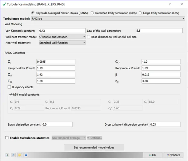
The RANS K-Epsilon model is selected as the turbulence model, with the values for the constants as shown below.
Grid size
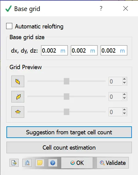
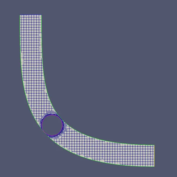
The base grid is defined with the required size along all three axes. The size here is 2e-3.
Fixed embedding at the throttle body are added for further mesh refinement.
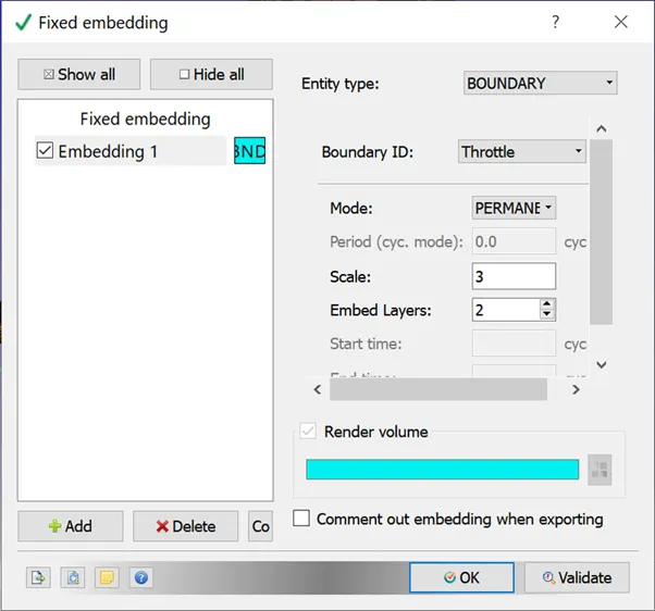
The output and post processing parameters are kept default, and the setup is completed for simulation.
The simulation is carried out using Cygwin, and the results are illustrated below.
Results
Grid size: dx - 2.0 e-3,dy - 2.0 e-3, dz - 2.0 e-3
Mass flow rate
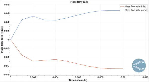
The mass flow rate at the inlet and the outlet are conserved, at around 0.065 kg/s, when the flow attains steady state. It can be seen, that during the throttling time (0.002 - 0.004s), the mass flow rate reduces, due to the reduced area when the throttle rotates, and again increases gradually before becoming steady again at 0.008s.
Velocity
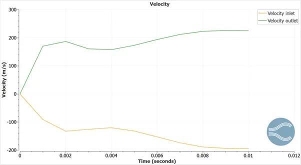
The velocity at the inlet is around -200 m/s. The peak velocity at the outlet is roughly 250m/s. The velocity increases because the flow is accelerated due to the throttle effect. It can be seen that the velocity reduces during the throttling time (0.002-0.004s) due to the throttle closing, and increases again as the throttle opens, and reaches a steady value at around 0.008s.
Pressure
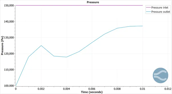
The pressure of 1.5 bar at the inlet remains constant. The pressure at the outlet increases, until it reaches a steady state value of around 1.4 bar. During the throttling time (0.002 - 0.004s), the pressure reduces due to backpressure of the throttle closing, and increases again as the throttle opens, until it reaches a steady value at around 0.008s.
Number of cells
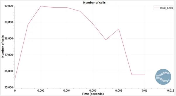
The number of cells increase as the throttle effect takes place. The number is not constant, since the mesh size is varying and the time step varies as the throttling action takes place. It reduces again and the mesh size at the end consists of roughly 36000 cells.
Results
Paraview
Mesh

Velocity contour
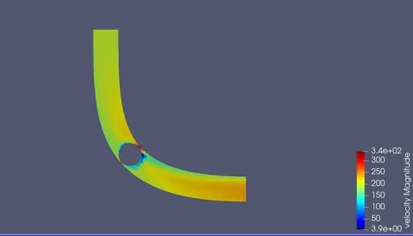
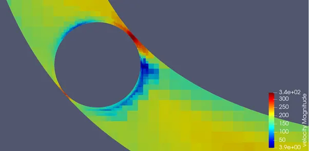
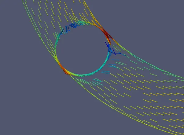
The velocity contour shows that the flow is accelerated in the small gap between the throttle body and the walls of the tube, since the area is reduced. The velocity is maximum in this region (red). There are stagnation regions ahead of and behind the throttle body, where the flow separation occurs. The velocity here is minimum (blue). This is also highlighted in the glyph plot below.
Pressure contour
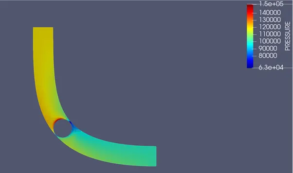
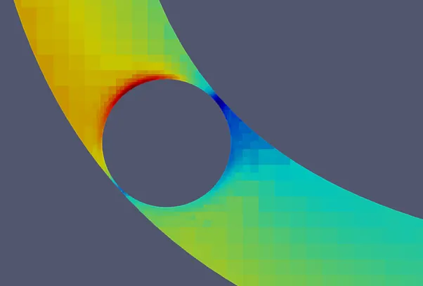
The pressure is lowest, at the gap between the throttle body and the walls (blue). This corresponds to the region where the velocity is maximum. The pressure is highest on the inlet face of the throttle body, where the flow separates and there is a stagnation point (red).
Animation pressure
Animation velocity
Conclusion
Thus the transient flow over a throttle body has been simulated and the results have been illustrated.