Week 9 - Mini project - Flow over an Airfoil
Objective
To simulate the flow over an airfoil for various angle of attacks and compare the effects of different turbulence models on the results.
Theory
An airfoil is the cross sectional shape of a wing, blade (of a propeller, rotor, or turbine). An airfoil shaped body moving through a fluid produces an aerodynamic force. The component of this force perpendicular to the direction of motion is called lift. The component parallel to the direction of motion is called drag. Subsonic flight airfoils have a characteristic shape with a rounded leading edge, followed by a sharp trailing edge, often with a symmetric curvature of upper and lower surfaces. Foils of similar functions designed with water as the working fluid are called hydro foils. An airfoil's lift coefficient can be increased by using flaps at the end of the airfoil without much increase in drag.
The lift on an airfoil is primarily the result of its angle of attack. Most foil shapes require a positive angle of attack to generate lift, but cambered airfoils can generate lift at zero angle of attack. This 'tuning' of the air in the vicinity of the airfoil creates curved streamlines, resulting in lower pressure on one side and higher pressure on the other. This pressure difference is accompanied by a velocity difference, via Bernoulli's principle. So the resulting flow field about the airfoil has a higher average velocity on the upper surface than on the lower surface.
Airfoil nomenclature
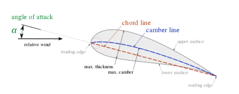
The geometry of the airfoil is described with a variety of terms
The leading edge is the point of the airfoil that has the maximum curvature (minimum radius).
The trailing edge is defined similarly as the point of maximum curvature at the rear of the airfoil.
The chord line is the straight line connecting leading and trailing edges.
The chord length, is the length of the chord line. That is the reference dimension of the airfoil section.
The shape of the airfoil is defined using the following geometrical parameters
The mean camber line is the locus of points midway between the upper and lower surfaces. Its shape depends on the thickness distribution along the chord
The thickness of an airfoil varies along the chord. It may be measured in either of two ways
- Thickness measured perpendicular to the camber line
- Thickness measured perpendicular to the chord line
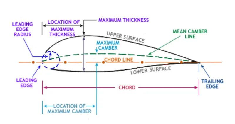
Common terms used to describe the airfoil's behaviour when it is moving through a fluid are
- The aerodynamic center is the chord wise length about which the pitching moment is independent of the lift coefficient and the angle of attack
- The center of pressure is the chord wise location about which the pitching moment is zero
Main types of NACA airfoil
The NACA four digit wing sections define the profile by
1. First digit - describing the maximum camber as a percentage of the chord
2. Second digit - describing the distance of maximum camber from the airfoil leading edge in tenths of the chord
3. Last two digits - describing the maximum thickness of the airfoil as a percent of the chord
For example - NACA 2412 airfoil has a total chord length of 100mm, So the airfoil has a maximum camber of 2mm which is 40 mm away from the leading edge with 12mm thickness.
Lift coefficient (Cl) - It is a dimensionless coefficient, that relates the lifting force on the body to its velocity, surface area and the density of the fluid in which it is lifting.
Lift force = `frac{1}{2}*Cunderset{l}{ } *rho*A*V^2`
Drag coefficient (Cd) - It is a dimensionless coefficient that relates the drag force on the body to its velocity, surface area, and the density of the fluid in which it is moving
Drag force = `frac{1}{2}*Cunderset{d}{ } *rho*A*V^2`
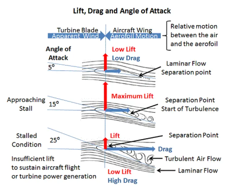
At very low angles of attack, the airflow over the airfoil is essentially smooth and laminar, with a small amount of turbulence occuring at the trailing edge of the airfoil. The point at which laminar flow ceases and turbulence begins is known as the separation point.
Increasing the angle of attack increases the area of the airfoil facing directly into the wind. This increases the lift, but it also moves the separation point of laminar flow of the air above the airfoil part way upwards towards the leading edge and results in increased turbulent flow and therefore increase in drag
Maximum lift occurs when the angle of attack is around 15 degrees, but it could be higher for specially designed airfoils.
Above 15 degrees, the separation point moves right up to the leading edge of the airfoil and the laminar flow above the airfoil is destroyed. The increased turbulence causes rapid deterioration of the lift force, while at the same time dramatically increasing the drag, resulting in a stall.
Solution
Geometry setup
The coordinates from the NACA airfoil website are taken, and input into an excel sheet. These coordinates are then entered into Solidworks using the "Curve through the XYZ" feature and the geometry is created.
The chord length for each case was taken as 50 mm.A virtual wind tunnel was setup with the following dimensions
Horizontal length of wind tunnel = 50 x chord length = 2.5m
Vertical length of wind tunnel = 30 x chord length = 1.5 m
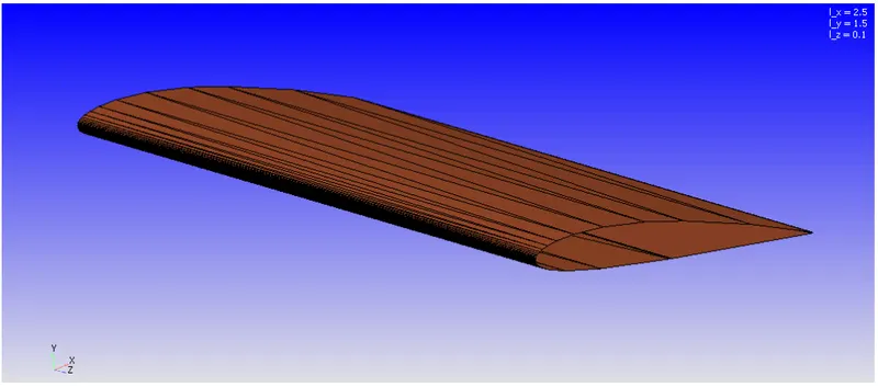
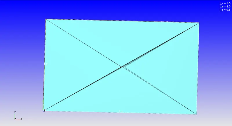
The box dimensions are
dx - 2.5m, dy - 1.5m, dz - 0.1m
The normals were transformed to point them inside the direction of the fluid region
Boundary creation
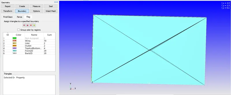
A total of 6 different boundaries were created for multiple split triangles of the geometry with each face split into multiple triangles.
Case setup
A time based simulation is selected, with Air as the predefined mixture. Default values are chosen for the global transport parameters and the species. Reaction mechanism (mech.dat) was selected for this case study.
Simulation parameters
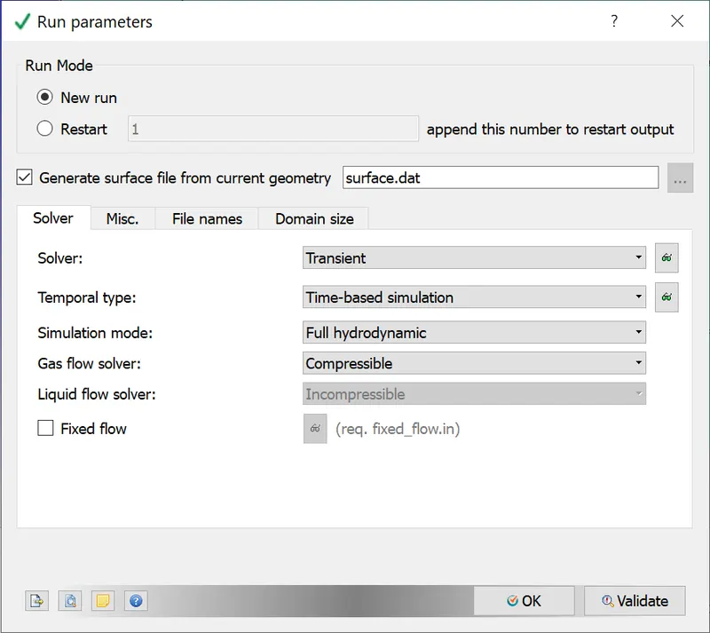
A transient solver was selected for running this case study along with a Density based solver
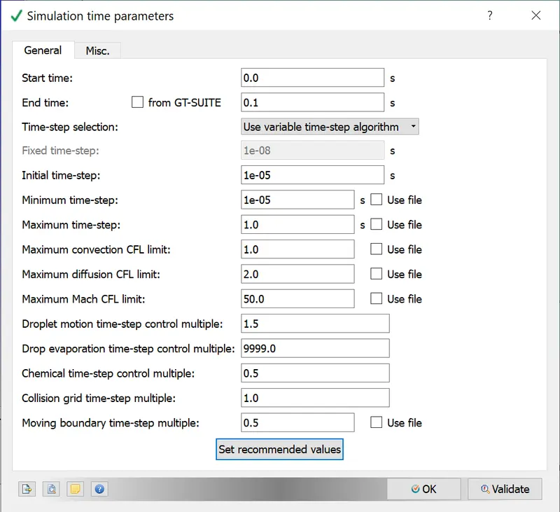
The end time is chosen based on the following calculation
Reynolds number = 200000
Density of air at 300 K `rho=1.766 frac{kg}{m^3}`
Dynamic viscosity at 300 K `mu =0.00001846 frac{kg}{ms}`
Kinematic viscosity `frac{mu}{rho}=1.56893 E-05 frac{m^2}{s}`
Characteristic length = 50 mm
Average flow velocity `frac{Re*mu}{rho.L}=60.8 frac{m}{s}`
Horizontal length = 2.5m
Speed = Distance/time. Therefore Time = 0.041s
We are simulating roughly two times of flow, ie 0.1s
Boundary conditions
| Boundary name | Boundary type | Parameter defined | Boundary ID |
| Inlet | Inflow | 60.8 m/s - X axis | 2 |
| Outlet | Outflow | 101325 Pa | 3 |
| Front 2D | TWO_D | 5 | |
| Back 2D | TWO_D | 6 | |
| Top and botto m wall | Symmetry | 4 | |
| Wings | wall | Law of wall |
1 |
Initial conditions and Events
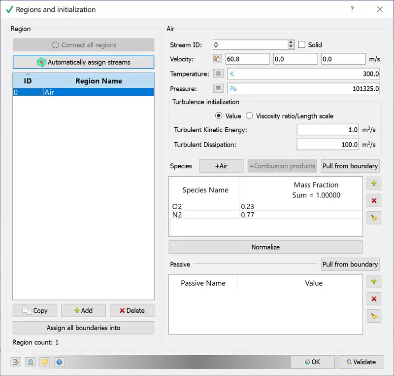
A volumetric regions was created in order to assign this to the boundary tags.
Species - O2 (0.23) and N2 (0.77)
Pressure - 101325 Pa
Temperature - 300K
Velocity - 60.8m/s - X axis
Physical models
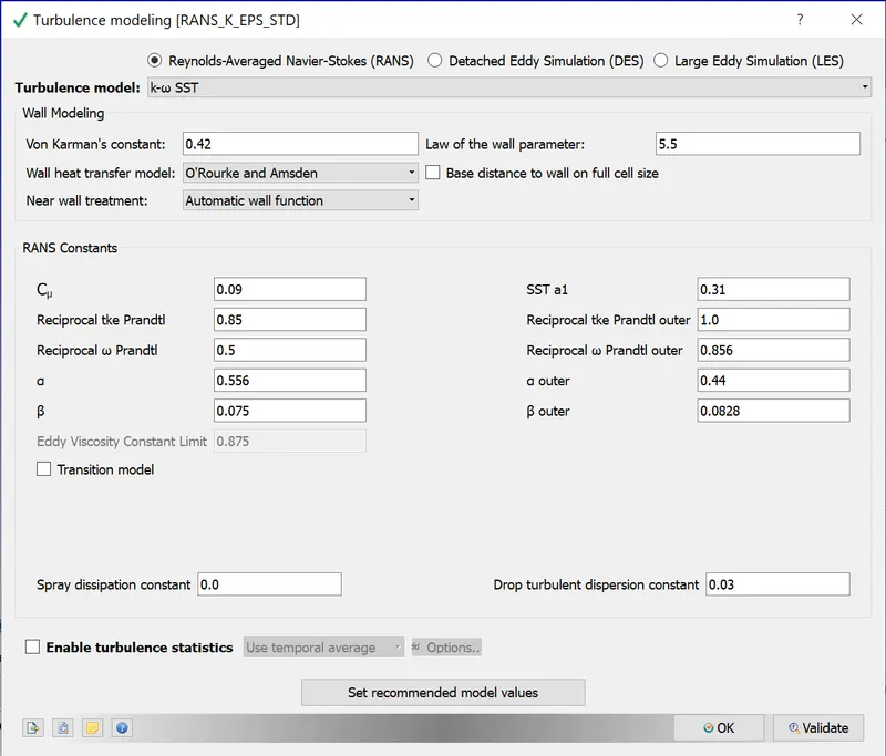
For the angle of attack of 1 degree, two different turbulent models are used for simulation
1. K-omega-SST
2. K-Epsilon
For all the other angle of attacks (5,10,15) K-omega-SST is used for simulation
1 K-omega-SST
Grid control
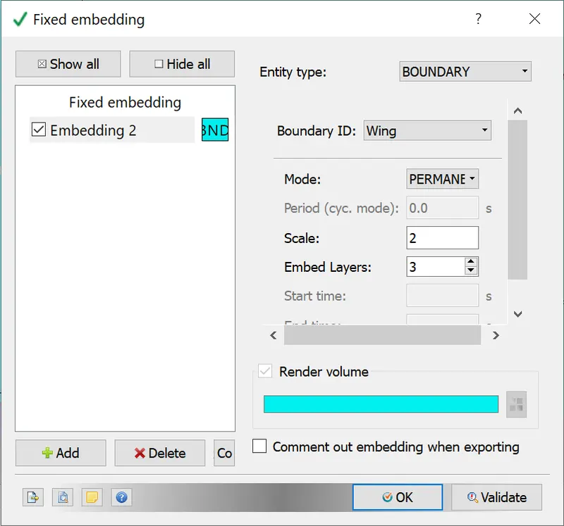
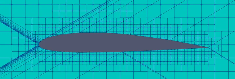
the mesh size is
dx - 0.004m, dy = 0.004m, dz - 0.004m
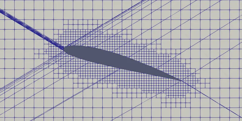
Fixed embedding was done in order to capture the edges of the airfoil better
Output/Post processing
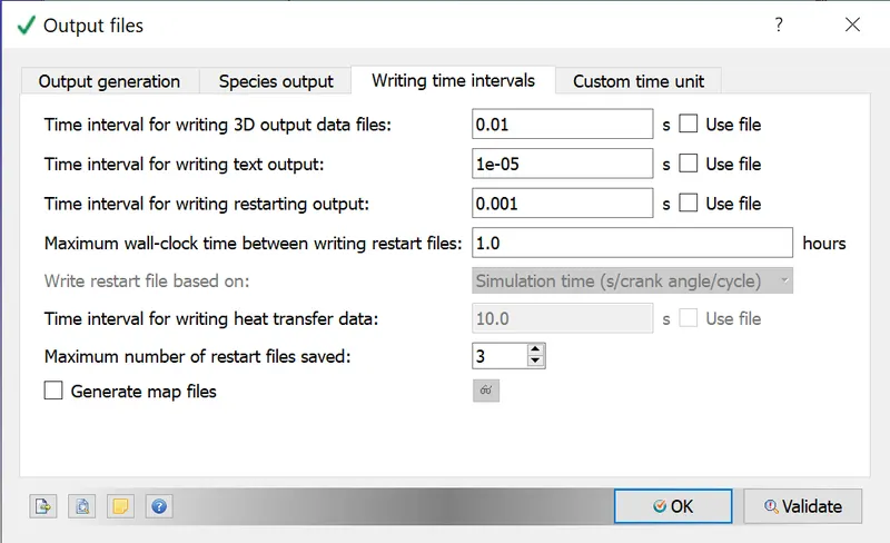
Time interval for writing the 3D output files - 0.01s
Time interval for writing restart files - 0.001s
The simulation was run using CYGWIN, and the post processing was done in ParaView.
Results
1. AOA - 1 degree
K-omega-SST model
Mesh
Velocity contour
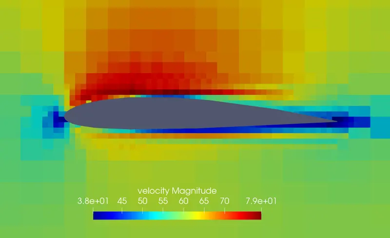
The velocity contour shows the presence of a stagnation point at the leading edge, when the velocity is lowest, and over the upper convex section of the wing, it increases, as the pressure is low. As the flow proceeds along the upper surface, it separates at a point, after which the velocity reduces.
Pressure contour
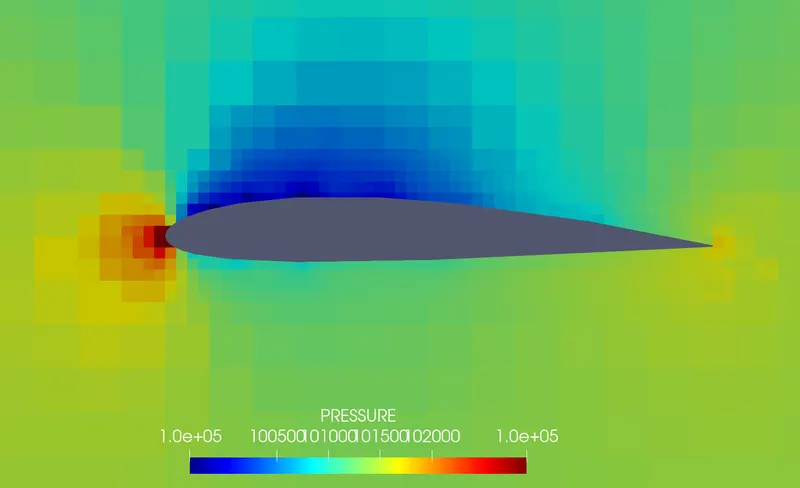
The pressure contour shows the presence of low pressure on the top surface of the wing, and higher pressure on the lower side. The net effect is a force that pushes the wing upwards, resulting in lift.
Animation velocity
Animation pressure
2. K-epsilon model
Velocity contour
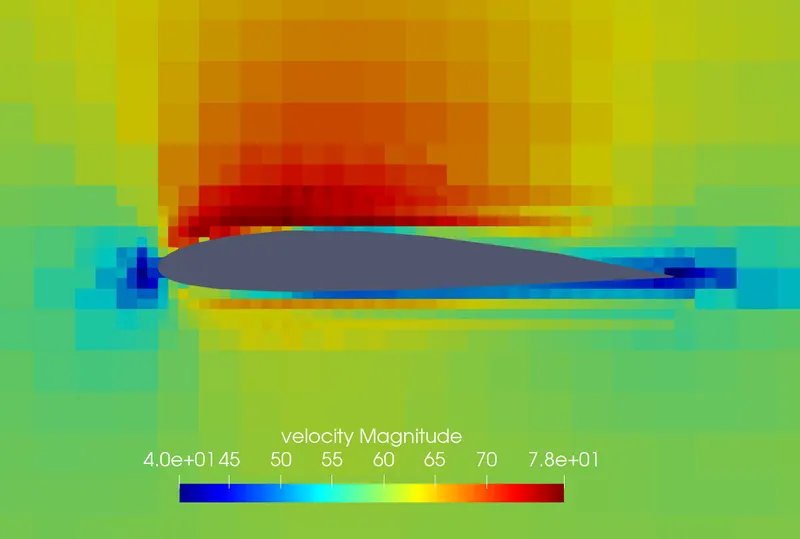
The velocity contour shows the presence of a stagnation point at the leading edge, when the velocity is lowest, and over the upper convex section of the wing, it increases, as the pressure is low. As the flow proceeds along the upper surface, it separates at a point, after which the velocity reduces.
Pressure contour
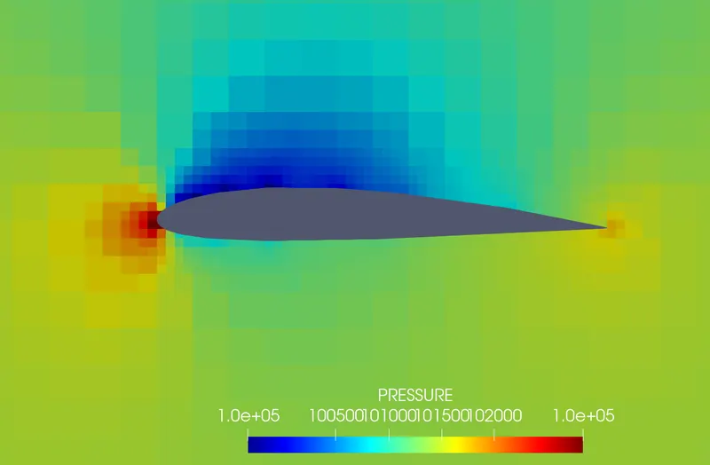
The pressure contour shows the presence of low pressure on the top surface of the wing, and higher pressure on the lower side. The net effect is a force that pushes the wing upwards, resulting in lift.
Animation velocity
Animation pressure
Comparison
Drag force
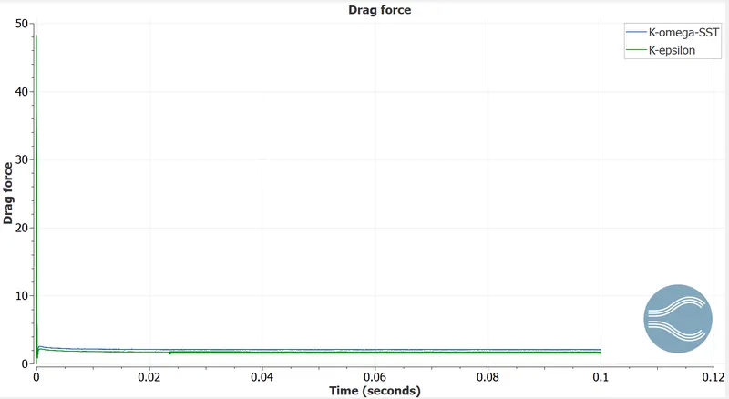
The magnitude of the drag force with the K-omega-SST is slightly lower than the K-epsilon model
Lift force
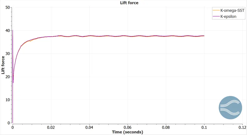
The magnitude of the lift force is almost equal with both models
Y plus avg
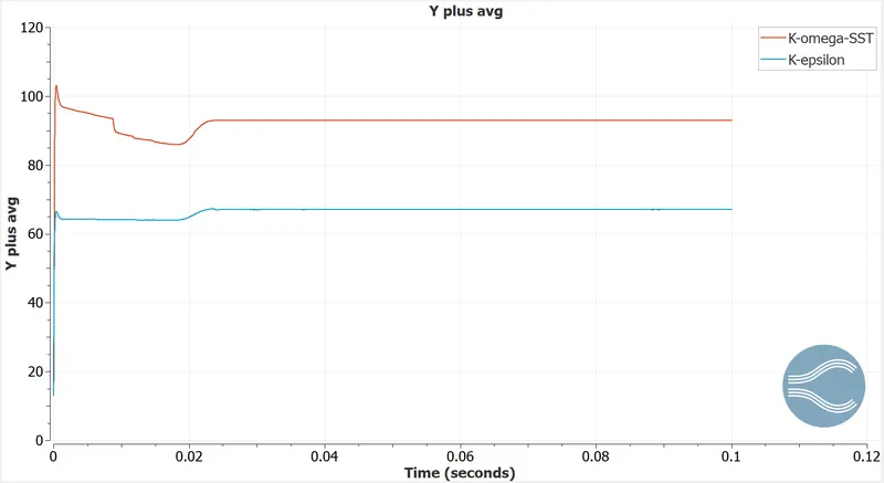
The Y plus avg of the K-omega model is significantly higher than the K-epsilon model. The K-omega SST has integrated wall treatment in its solver, which makes it more suitable for large Reynolds number simulations.
Using the lift and the drag forces, the lift and drag coefficients can be calculated according to the equations
Fl = `frac{1}{2}*Cunderset{l}{ } *rho*A*V^2`
Fd = `frac{1}{2}*Cunderset{d}{ } *rho*A*V^2`
The area A = 0.05 * 0.1 = 0.005 m^2.
| S.no | Turbulence model | Lift force (N) | Lift coefficient | Drag force (N) | Drag coefficient | Y plus avg |
| 1 | K-omega-SST | 37.354 | 2.28 | 2.07 | 0.12 | 92.97 |
| 2 | K-epsilon | 37.605 | 2.3 | 1.764 | 0.108 | 67.05 |
The results of the simulations of the other angles of attack are illustrated below.
2. AOA - 5 degrees
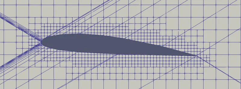
Mesh
Velocity contour
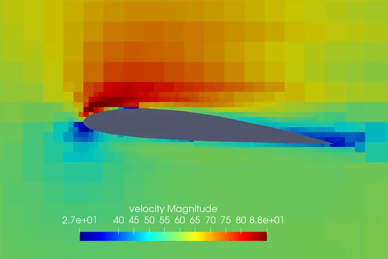
It can be seen, that the magnitude of the velocity has increased compared with an AOA of 1 deg. But the flow separation point has moved forward significantly, which means that the flow over the wing on the upper surface becomes turbulent faster.
Pressure contour
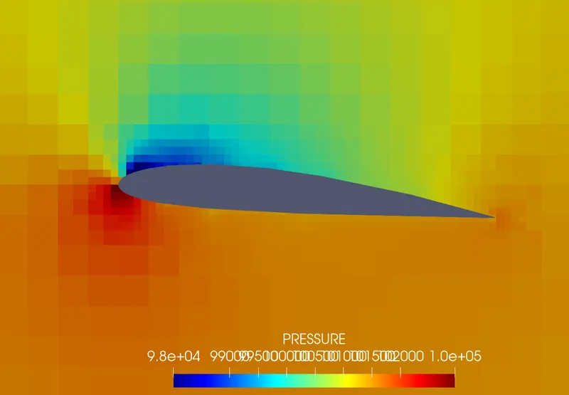
The region of low pressure on the top surface of the wing has reduced to a small region near the leading edge. The pressure on the underside of the wing is higher, resulting in a net lift.
Animation velocity
Animation pressure
3. AOA - 10 degrees
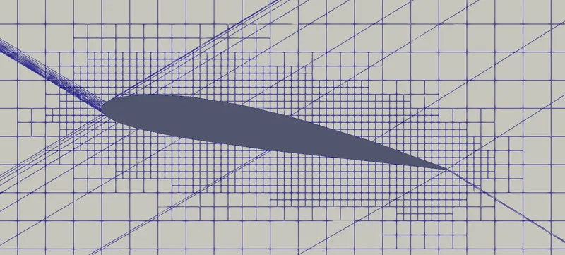
Mesh
Velocity contour
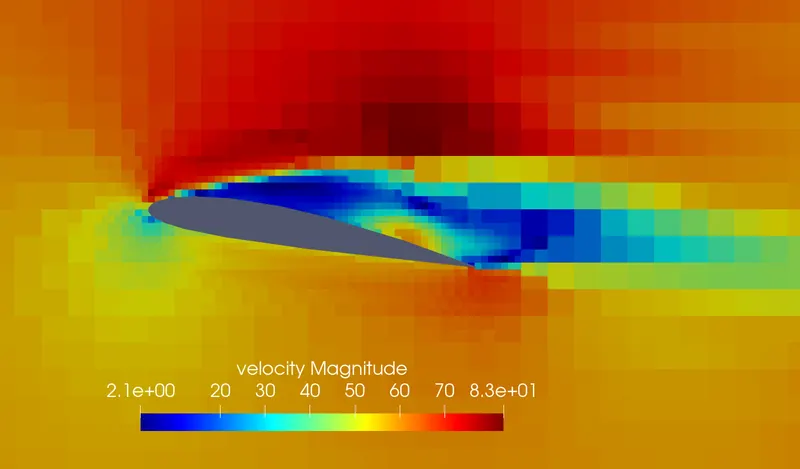
The flow starts separating virtually at the leading edge itself, and the stream on the upper surface has become very turbulent.
Pressure contour
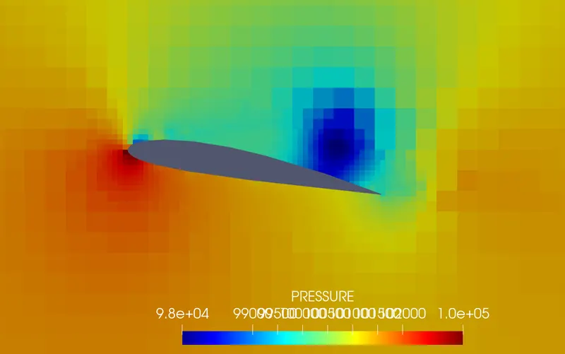
The presence of a recirculation region on the top surface of wing near the trailing edge leads to very low pressure.
Animation velocity
Animation pressure
3. AOA - 15 degrees
Mesh
Velocity contour
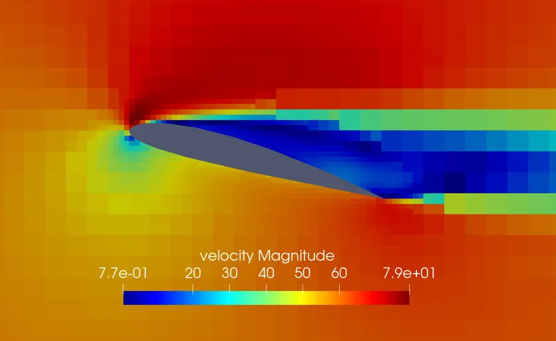
The flow has stalled, which means that the velocity of the stream close to the wing is extremely low, and the lift generated is correspondingly reduced.
Pressure contour
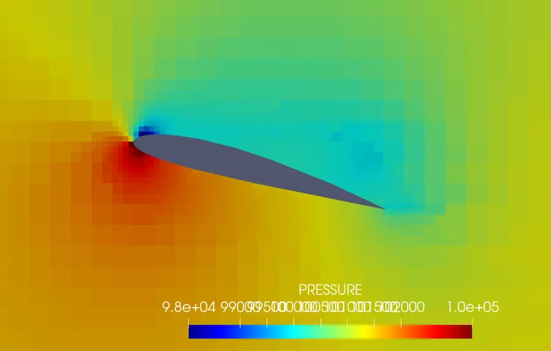
At the stall point, the pressure is low on the upper side and high on the under side. The drag force increases tremendously, with no corresponding lift gain.
Animation velocity
Animation pressure
Comparison
Y plus avg
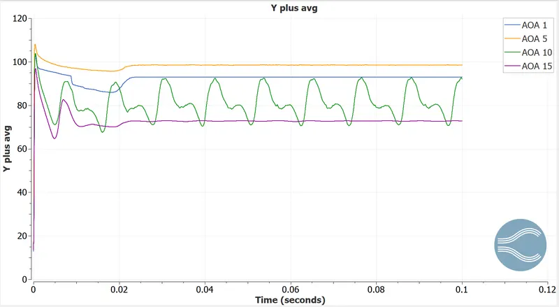
Lift and drag coefficient calculation

Lift force
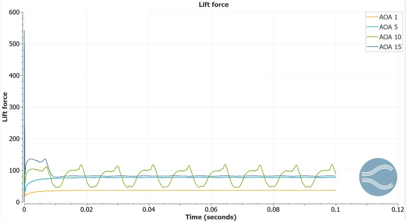
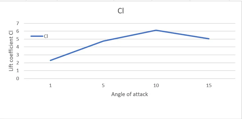
It can be seen, that the lift force increases with angle of attack until 10 degrees, as the velocity on the upper surface of the wing increases. Thereafter, the separation point moves to the front of the wing, where the flow stalls, as the angle of attack is further increased. This reduces the lift force produced, and increasing the angle of attack after this point has no effect.
Drag force
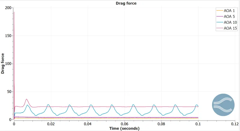
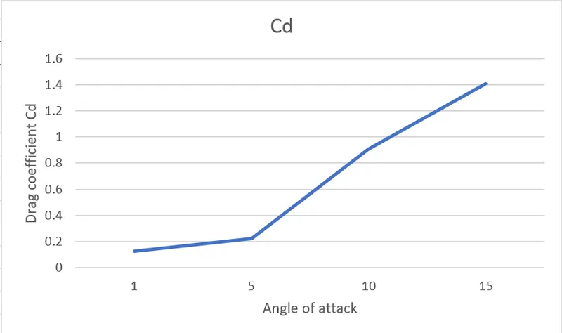
The drag force increases, as the angle of attack is increased, since an increase of lift force is always accompanied by an increase of drag. After an angle of attack of 10 degrees, the drag force increases tremendously, even as the lift force reduces due to stall. This happens due to increased flow separation at the very beginning of the wing, and the flow is extremely turbulent.
Conclusion
Thus the flow over an airfoil for different angle of attacks has been simulated, and the effect of different turbulence models have been discussed.