Week 1: Channel flow simulation using CONVERGE CFD
Objective
To perform the channel flow simulation using three different mesh sizes, and to compare the post processed results from.
Solution
Geometry creation - Converge
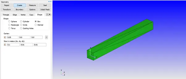
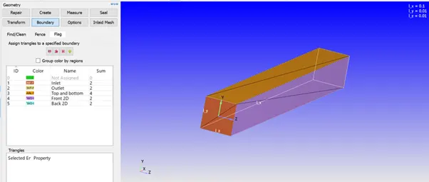
The geometry is created using the measurements shown in the figure below
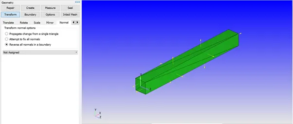
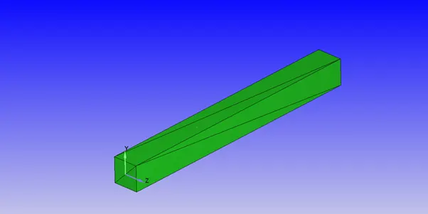
The direction of the normals are reversed, such that they point inwards, since the flow happens inside the channel
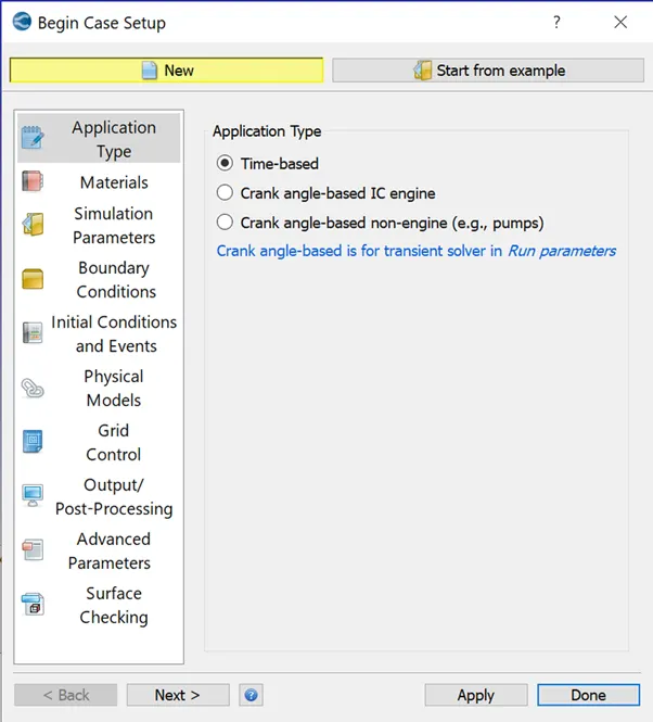
The first step in the case setup is to choose a time based simulation
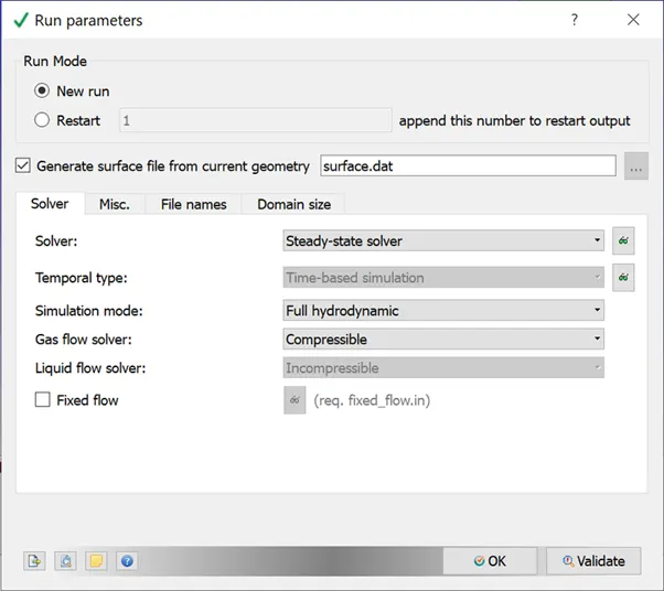
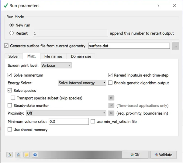
The steady state solver is selected and the use shared memory check box is unchecked
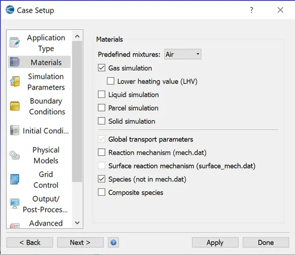
Air is selected as the medium, and the other fields and the global transport properties are kept default
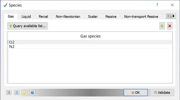
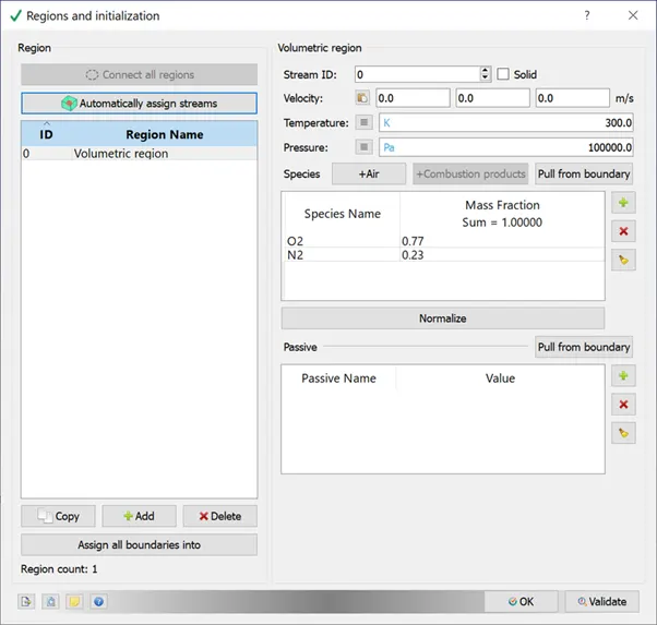
Under species, O2 and N2 are selected
The boundaries are assigned to the sides of the geometry as follows
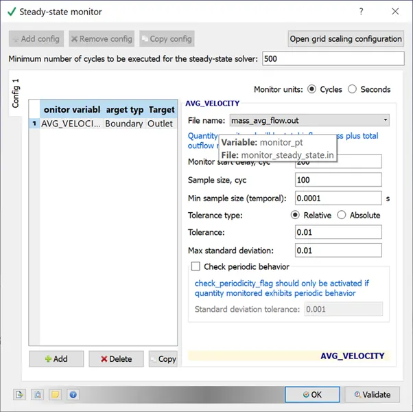
Under run parameters, steady state monitor is checked, and the parameter to be monitored is given as the average velocity.
The start and end cycles are defined in the steady state monitor, along with the target boundary. In this case, the outlet is selected
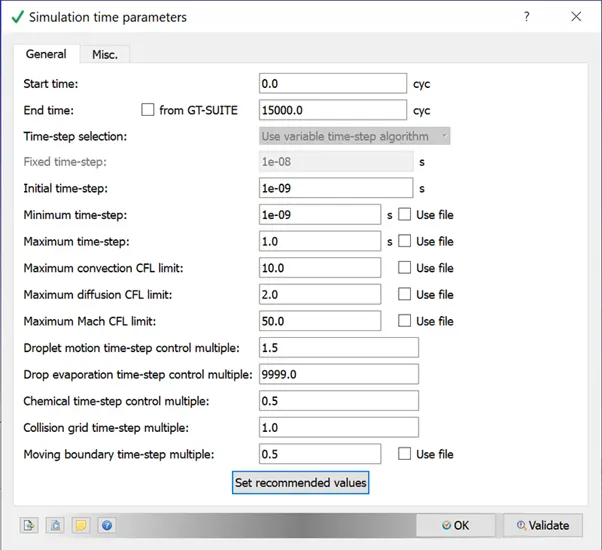
The default values are used for the simulation time parameters. The end time is 15000 cycles
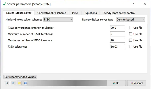
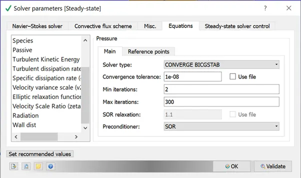
A Navier stokes density based solver is selected, and under the equations tab, the preconditioner for pressure is selected as SOR
The boundary conditions are defined for each boundary as shown below
Inlet
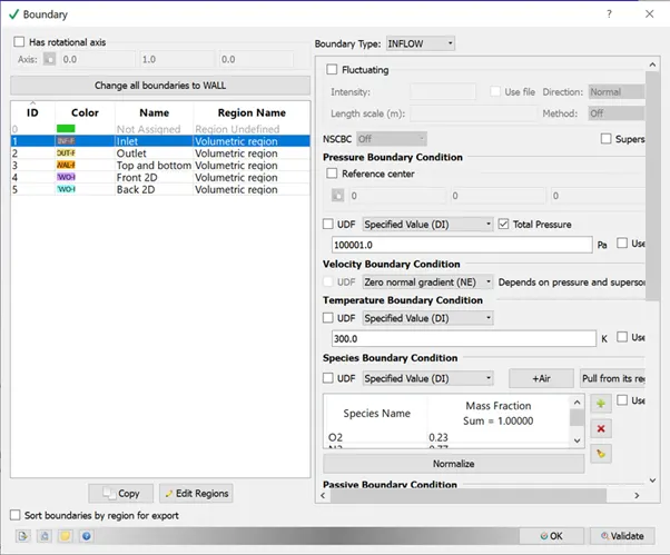
Outlet
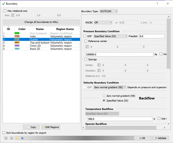
Top and Bottom
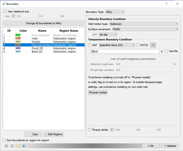
The front and back are defined as 2D walls.
The flow region is initialized with the components of air, and the temperature and pressure
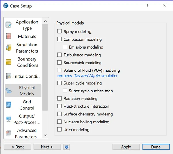
Under physical models, turbulence modeling is unchecked
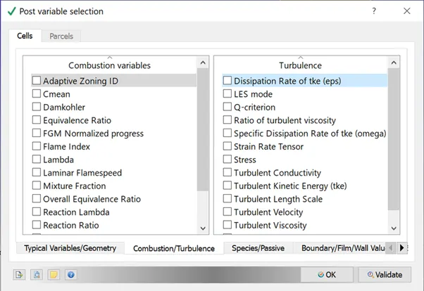
Under post variable selection, all turbulence tabs are unchecked
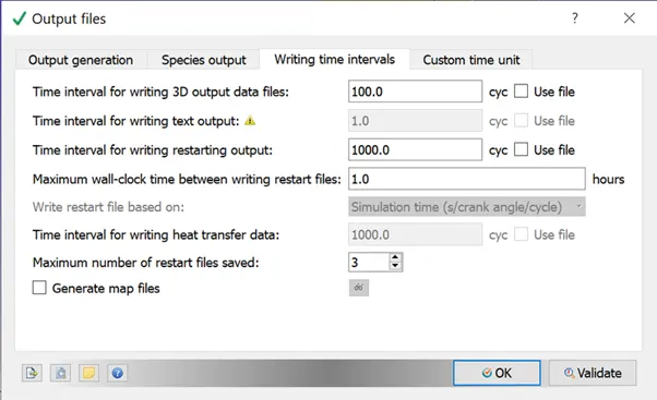
The time intervals for writing output files are defined, and the case setup is complete
The required grid size can be defined in base grid, and the simulation can be performed.
Results
- Grid size: dx = 2e-4, dy = 2e-4, dz = 2e-4
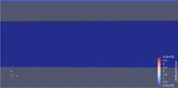
Mesh
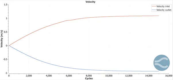
Velocity
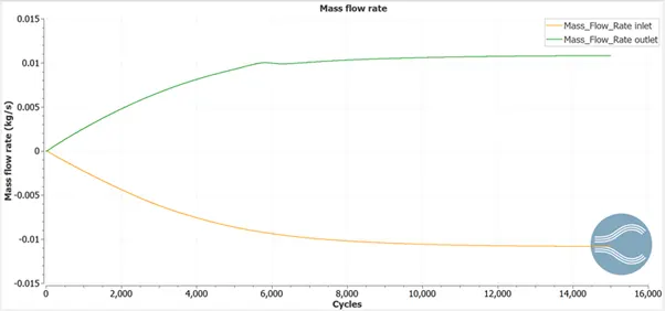
Mass flow rate
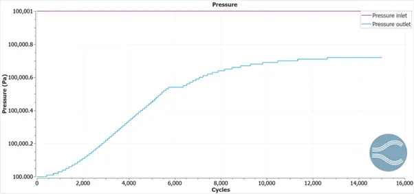
Pressure
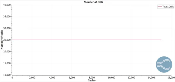
Number of cells
Paraview
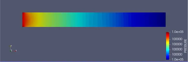
Pressure contour
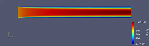
Velocity contour
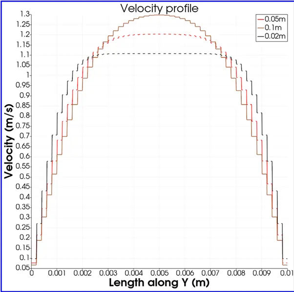
Velocity profile
Observation
The velocity profiles at three different regions along the length of the tube show slight differences. At the entrance (0.02m) the velocity profile is not fully formed, due to the influence of the boundary layer. The peak velocity here is 1.1m/s. At the midpoint (0.05m)the peak velocity is 1.2 m/s, and reaches the peak of 1.3m/s at the end length of the tube (0.1m).
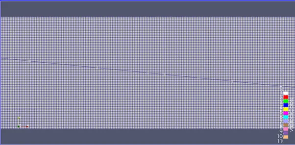
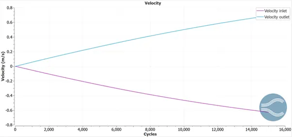
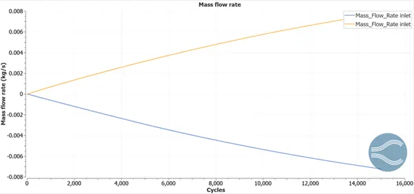
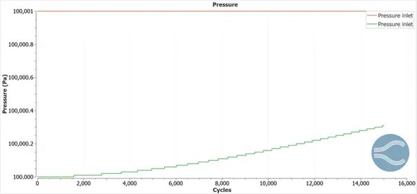
- Grid size: dx = 1.5e-4, dy = 1.5e-4, dz = 1.5e-4
Mesh
Velocity
Mass flow rate
Pressure
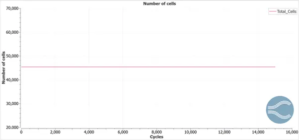
Number of cells
Paraview
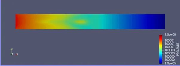
Pressure contour
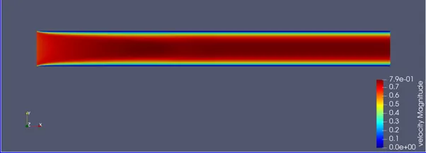
Velocity contour
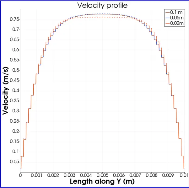
Velocity profile
Observation
The velocity profiles at three different regions along the length of the tube show slight differences. At the entrance (0.02m) the velocity profile is not fully formed, due to the influence of the boundary layer. At the midpoint (0.05m) it is fully formed, and remains constant throughout the length of the tube (0.1m).
- Grid size: dx = 1e-4, dy = 1e-4, dz = 1e-4
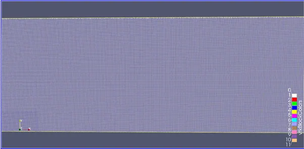
Mesh
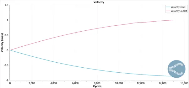
Velocity
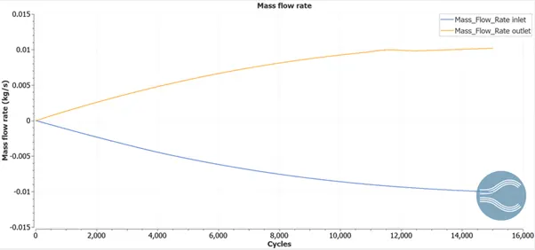
Mass flow rate
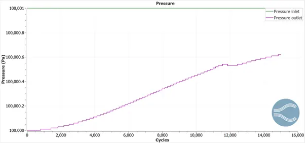
Pressure
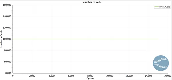
Number of cells
Paraview
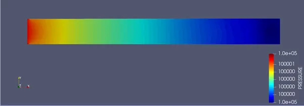
Pressure contour
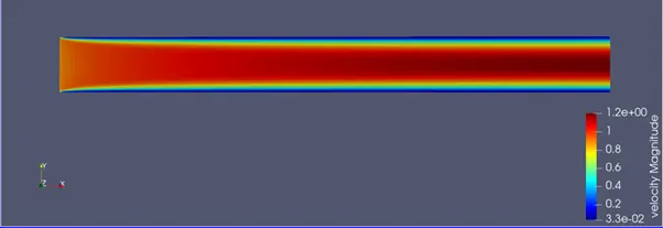
Velocity contour
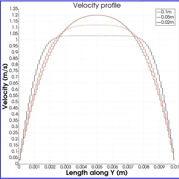
Velocity profile
Observation
The velocity profiles at three different regions along the length of the tube show slight differences. At the entrance (0.02m) the velocity profile is not fully formed, due to the influence of the boundary layer. At the midpoint (0.05m)the peak velocity is 1.15 m/s, and reaches the peak of 1.25m/s at the end length of the tube (0.1m).
Conclusion
Thus the simulation has been performed for three different mesh sizes, and the results have been illustrated and compared.
Animation link of velocity for Mesh size of 2e-4
Animation link of pressure for Mesh size of 2e-4