Week 11: FSAE Car Project

Objective

To simulate the airflow around an FSAE car for two different scenarios and analyze the results.

Geometry clean up - Converge

The stl file is imported into Converge, and scaled to transform units from inches to metres. The model is then checked for geometry errors.

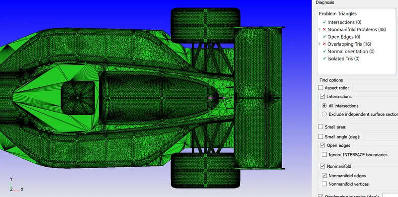
There are 48 errors arising from non-manifold edges. These errors are cleaned using the Repair - Delete, Patch and Stitch options.

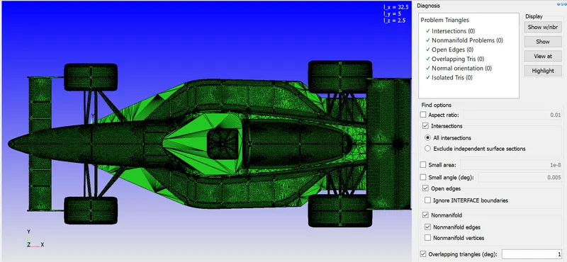
The normal orientation was fixed, and the geometry is now ready for boundary flagging.

Boundary creation

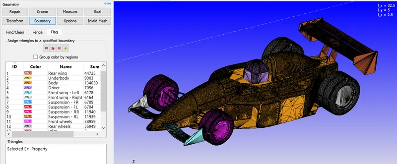
The geometry was split into 12 different boundaries as shown below.

Virtual wind tunnel

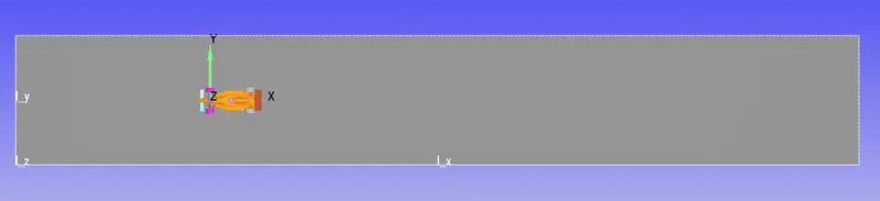
A virtual wind tunnel with the following dimensions were created.

dx = 32.5m

dy = 5m

dz = 2.5m

The distance in front of the car is around 3 times the wheelbase = 3*2.5 = 7.5m

The distance behind the car is 10 times the wheelbase = 10*2.5 = 25m

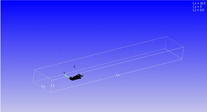
For case 1, the final wind tunnel setup looks like this

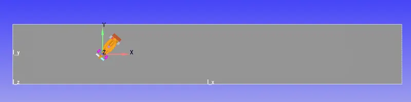
For case 2, the car was rotated according to the following calculation

70% turns at 45 degrees

20% turns at 80 degrees

10% turns at 20 degrees

Weighted average = `frac{0.70*45+0.20*80+0.10*20}{0.70+0.80+0.20} = 49.5 deg`

Case setup

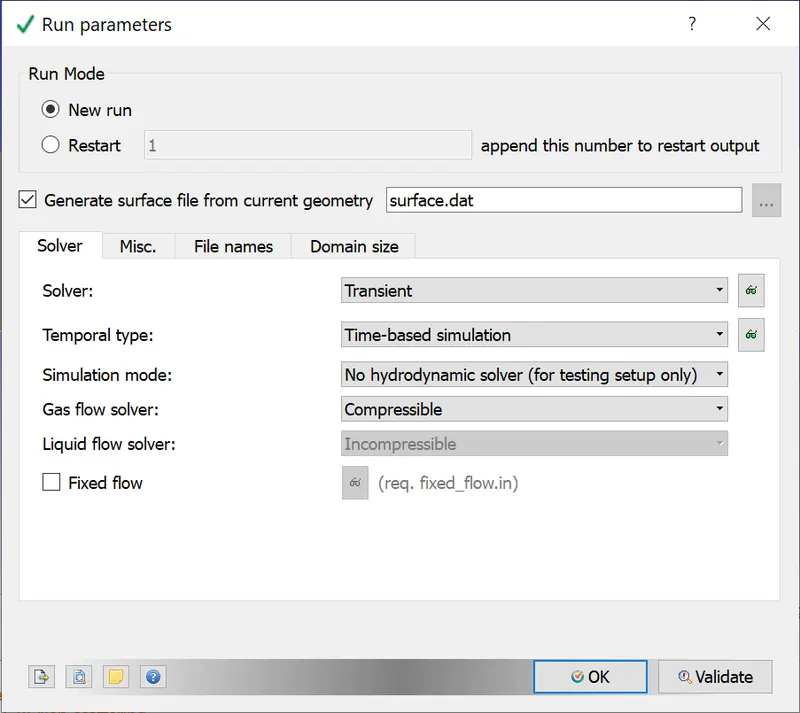
A time based simulation is selected with Gas simulation and Air as the predefined mixture.

The default values are used for the global transport parameters.

Simulation parameters

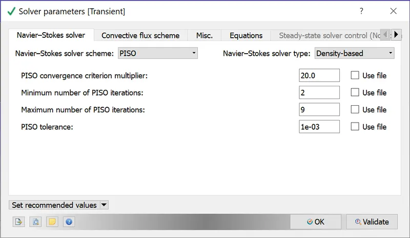
A transient, density based, PISO solver is selected.

A no hydrodynamic case is first run, to check for errors in the case setup

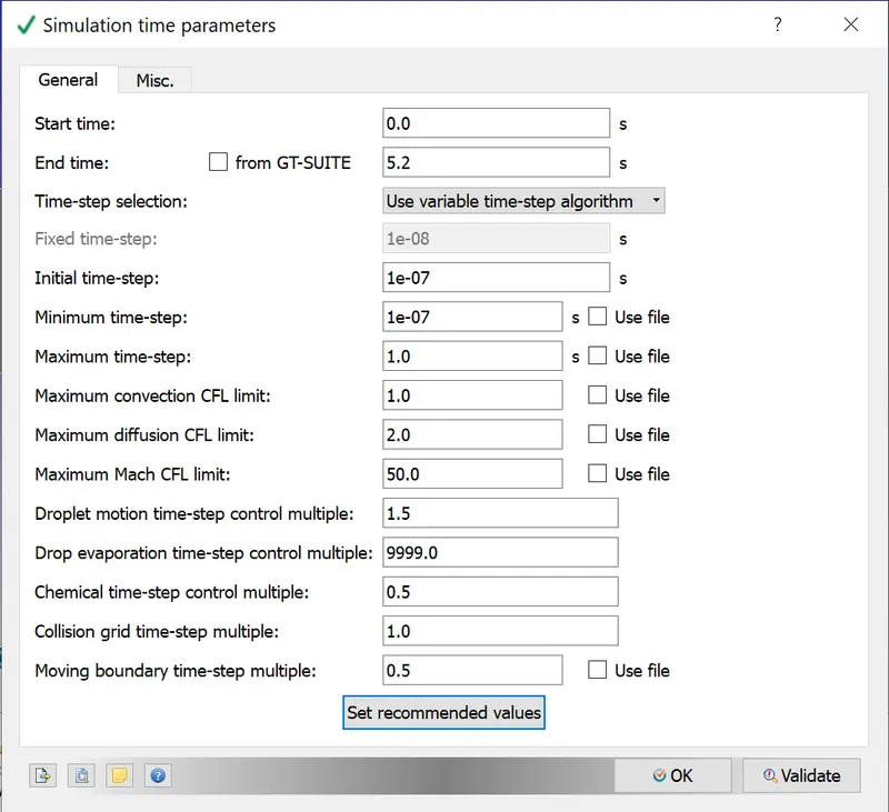
Calculation of time

Length = 32.5m

Average velocity (given) = 45 km/hr = 12.5 m/s

Speed = Distance/time

Therefore time = 2.6 s

We are simulating roughly 2 times of flow - 5.2 s

Boundary conditions

The boundary conditions for each boundary are defined as follows

S.No	Boundary_name	Boundary_type	Value	Boundary ID
1	Rear wing	Wall	Law of wall	1
2	Underbody	Wall	Law of wall	2
3	Body	Wall	Law of wall	3
4	Driver	Wall	Law of wall	4
5	Front wing - Left	Wall	Law of wall	5
6	Front wing - Right	Wall	Law of wall	6
7	Suspension - FR	Wall	Law of wall	7
8	Suspension - FL	Wall	Law of wall	8
9	Suspension - RL	Wall	Law of wall	9
10	Suspension - RR	Wall	Law of wall	10
11	Front wheels	Wall	Law of wall	11
12	Rear wheels	Wall	Law of wall	12
13	Inlet	Inflow	Pressure - NE Velocity - 12.5 m/s in X direction	13
14	Symmetry	Symmetry		14
15	Outlet	Outflow	Pressure - 101325 Pa Velocity - NE	15
16	Bottom wall	Wall	Law of wall	16

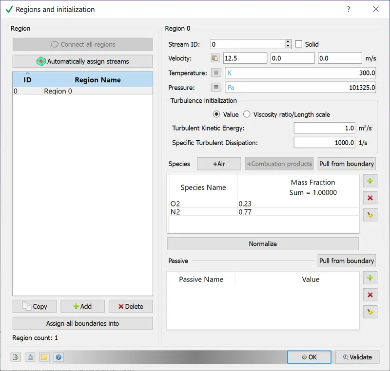
Initial conditions and Events

A volumetric regions was created in order to assign this to the boundary tags.

Species - O2 (0.23) and N2 (0.77)

Pressure - 101325 Pa

Temperature - 300K

Velocity - 12.5m/s - X axis

Physical models

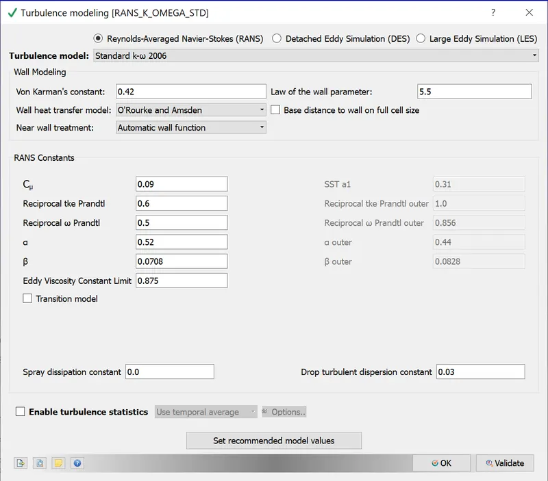
A standard K-omega model with default parameters is selected.

Grid control

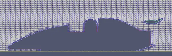
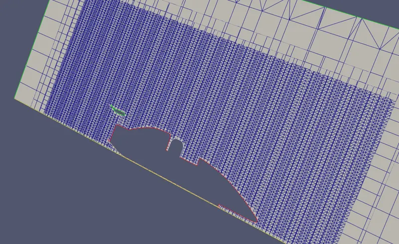
The mesh size is

dx - 0.5m, dy = 0.5m, dz - 0.5m

A coarse mesh is used to reduce computational time.

Output/Post processing

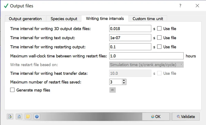
Time interval for writing the 3D output files - 0.018s

Time interval for writing restart files - 0.1s

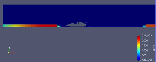
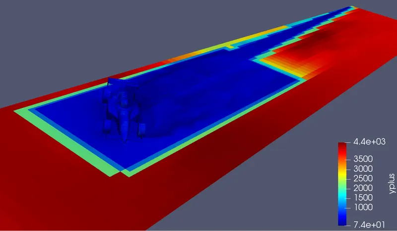
Under the post variables, vorticity and y+ are also selected.

The simulation was run using CYGWIN, and the post processing was done in ParaView.

Results

Case 1: Straight

Mesh

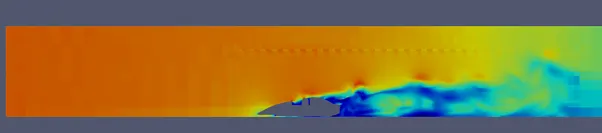
Velocity contour

Y plus

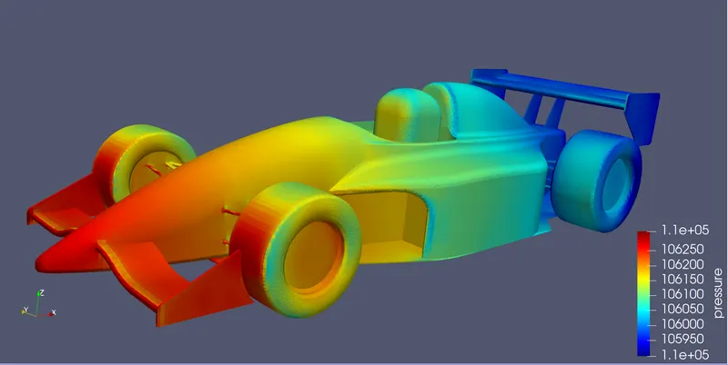
Pressure contour

Calculation of lift and drag forces

The lift and drag forces can be calculated in Paraview by extracting the surface and generation of surface normals.

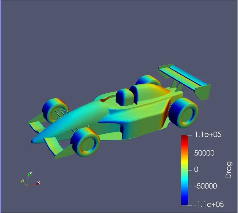
Drag

The pressure is multiplied by normals along X for calculating drag, as shown below.

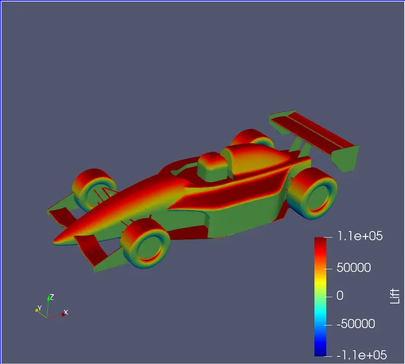
Lift

The pressure is multiplied by normals along Z for calculating lift, as shown below.

The values of lift and drag can be found by integrating the cell variables, as shown below.

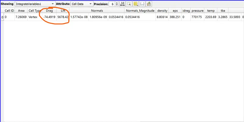
Drag force = -75 N

Lift force (downforce) = 5678 N

Results

Case 2: Turn

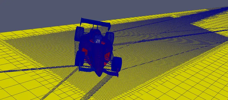
Mesh

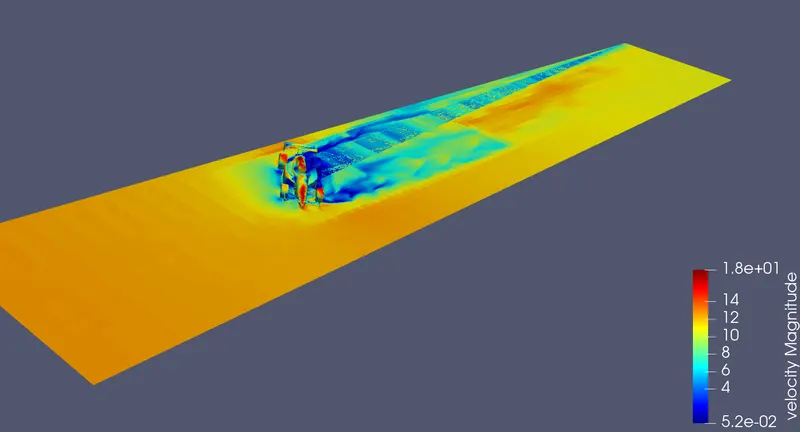
Velocity contour

Y plus

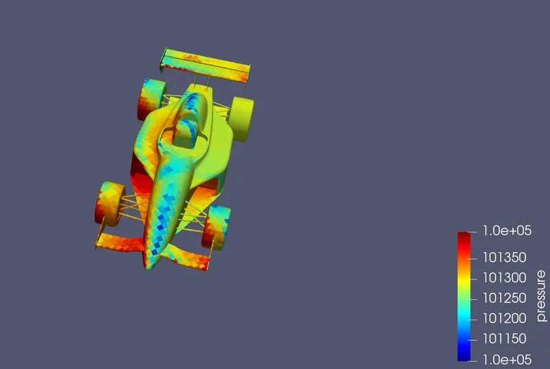
Pressure contour

Calculation of lift and drag forces

The lift and drag forces can be calculated in Paraview by extracting the surface and generation of surface normals.

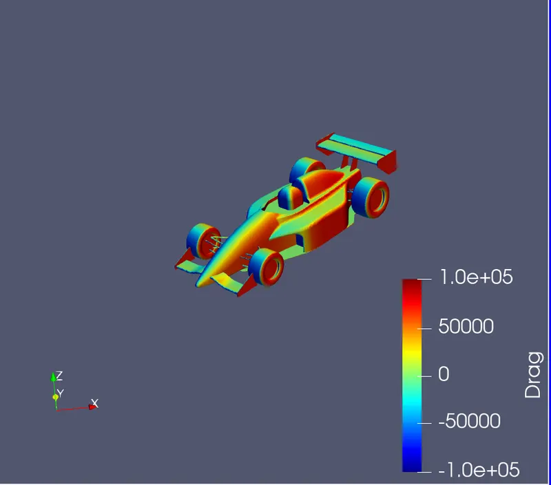
Drag

The pressure is multiplied by normals along X for calculating drag, as shown below.

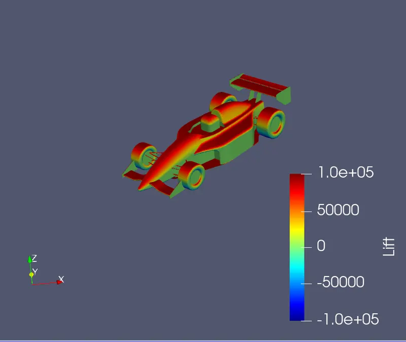
Lift

The pressure is multiplied by normals along Z for calculating lift, as shown below.

The values of lift and drag can be found by integrating the cell variables, as shown below.

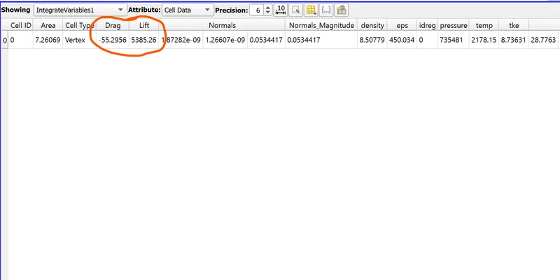
Drag force = -55 N

Lift force (downforce) = 5385 N

Conclusion

Thus the simulation has been done for both cases, and the results have been illustrated.