Week 3.5 - Deriving 4th order approximation of a 2nd order derivative using Taylor Table method

Aim:

To derive the fourth order approximations of the second order derivative using the central difference, skewed right hand, and skewed left hand schemes and compare them with the results of the analytical derivative.

Function : `f(x) = e^x cos(x)`

Analytical first derivative: `f'(x) = e^x (cos(x) -sin(x))`

Analytical second derivative: `f''(x) = - 2 e^xsin(x)`

Numerical stencil for approximation schemes

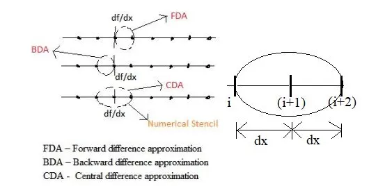
The figure shows the numerical stencil for forward, backward and central difference approximation schemes.

If we have to compute the second derivative `(del^2f)/(delx^2)`, with 2nd order accuracy using i,i+1 and i+2, then the numerical stencil is skewed.

Therefore we have skewed right handed, and skewed left handed schemes.

Central differencing scheme

Consider the following numerical stencil around point i.

For computing the second derivative at point i, the central difference scheme uses two values to the right (i+1),(i+2) and two values to the left (i-1) and (i-2).

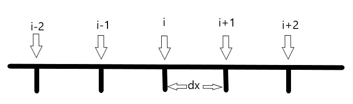
Let the hypothesis function be

`(del^2f)/(delx^2) = (a*f(i-2)+b*f(i-1)+c*f(i)+d*f(i+1)+e*f(i+2))`

Using the taylor's table, the coefficients can be computed as shown below

Coefficients	f(i)	`Deltax f'(i)`	`Deltax^2f''(i)`	`Deltax^3f'''(i)`	`Deltax^4.f^(IV)(i)`	`Deltax^5f^(V)(i)`	`Deltax^6f^(VI)(i)`
a.f(i-2)	a	-2a	(4/2)*a	-(8/6)*a	(16/24)*a	-(32/120)*a	(64/720)*a
b.f(i-1)	b	-b	b/2	-b/6	b/24	-(b/120)	b/720
c.f(i)	c	0	0	0	0	0	0
d.f(i+1)	d	d	d/2	d/6	d/24	d/120	d/720
e.f(i+2)	e	2e	(4/2)*e	(8/6)*e	(16/24)*e	(32/120)*e	(64/720)*e
Sum	0	0	1	0	0	?	?

The sum of the `Deltax^2f''(i)` is equal to one, and the rest of the sums are zero until the 5th order. The sums of the last two are unknown. Considering the terms until 5th order, we have 5 equations with 5 unknowns.

1. a+b+c+d+e = 0

2. -2a - b +d + 2e = 0

3. 2a + b/2 + d/2 + 2e = 1

4. -(4/3)a - b/6 + d/6 + (4/3)e = 0

5. (2/3)a + b/24 + d/24 + (2/3)e = 0

These equations can be converted into a matrix form, and solved in Matlab to find the 5 coefficients.

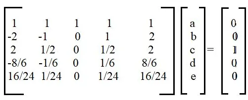
By solving the equations, we get

a = -0.0833

b = 1.3333

c = -2.5000

d = 1.3333

e = -0.0833

Also a=e, b=d

Using these values in the equations above in 1-5, the sum of equation 3 is 1, and the sum of the rest are zero.

Also, applying these coefficients to the fifth and sixth order coefficients, the sum of 5th order coefficients is zero, and sixth is non zero.

Therefore, the equation can be rewritten as

`(∂^2 f)/(∂x^2) = (a*f(i-2)+b*f(i-1)+c*f(i)+d*f(i+1)+e*f(i+2)) ≅Deltax^2f'' (x)+∆x^6 f^6(x)(CONSTANT)`

Dividing by `Deltax^2`we have

`(∂^2 f)/(∂x^2)=(a*f(i-2)+b*f(i-1)+c*f(i)+d*f(i+1)+e*f(i+2))/(∆x^2)≅f'' (x)+∆x^4 f^6(x)(CONSTANT)`

Here we can see, that the error term is of order 4. This is therefore, a fourth order approximation scheme.

Skewed right handed scheme

Consider the following numerical stencil around point i.

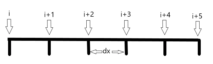
Let the hypothesis function be

`(del^2f)/(delx^2) = (a*f(i)+b*f(i+1)+c*f(i+2)+d*f(i+3)+e*f(i+4)+h*f(i+5))`

Using the taylor's table, the coefficients can be computed as shown below

Coefficients	f(i)	`Deltax f'(i)`	`Deltax^2f''(i)`	`Deltax^3f'''(i)`	`Deltax^4.f^(IV)(i)`	`Deltax^5f^(V)(i)`	`Deltax^6f^(VI)(i)`
a.f(i)	a	0	0	0	0	0	0
b.f(i+1)	b	b	b/2	b/6	b/24	(b/120)	b/720
c.f(i+2)	c	2c	(4/2)*c	(8/6)*c	(16/24)*c	(32/120)*c	(64/720)*c
d.f(i+3)	d	3d	(9/2)*d	(27/6)*d	(81/24)*d	(243/120)*d	(729/720)*d
e.f(i+4)	e	4e	(16/2)*e	(64/6)*e	(256/24)*e	(1024/120)*e	(4096/720)*e
h.f(i+5)	h	5h	(25/2)*h	(125/6)*h	(625/24)*h	(3125/120)*h	(15625/720)*h
Sum	0	0	1	0	0	?	?

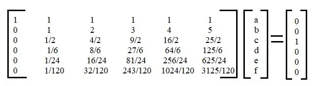
`he sum of the `Deltax^2f''(i)` is equal to one, and the rest of the sums are zero until the 5th order. The sums of the last two are unknown. Considering the terms until 5th order, we have 6 equations with 6 unknowns`

1. a+b+c+d+e+h = 0

2. b + 2c + 3d + 4e + 5h= 0

3. b/2 + (4/2)c + (9/2) d/2 + (16/2) e + (25/2)*h = 1

4. -b/6 + (8/6)*c + (27/6)*d + (64/6)*e + (125/6)*h = 0

5. b/24 + (16/24)*c + (81/24)* d + (256/24)*e + (625/24) * h = 0

6. b/120 + (32/120)* c + (243/120)*d + (1024/120)*e + (3125/120)*h=0

These equations can be converted into a matrix form, and solved in Matlab to find the 6 coefficients.

By solving the equations, we get

a = 3.7500

b = -12.8333

c = 17.8333

d = -13.0000

e = 5.0833

h = -0.8333

Using these values in the equations above in 1-6, the sum of equation 3 is 1, and the sum of the rest are zero.

Also, applying these coefficients to the sixth order coefficients, the sum of 6th order coefficients is non zero.

Therefore, the equation can be rewritten as

`(∂^2 f)/(∂x^2) = (a*f(i)+b*f(i+1)+c*f(i+2)+d*f(i+3)+e*f(i+4)+g*f(i+5))≅∆x^2 f''(x)+∆x^6 f^6(x)(CONSTANT)`

Dividing by `Deltax^2`we have

`(∂^2 f)/(∂x^2) = (a*f(i)+b*f(i+1)+c*f(i+2)+d*f(i+3)+e*f(i+4)+g*f(i+5))/(∆x^2)≅f''(x)+∆x^4 f^6(x)(CONSTANT)`

Here we can see, that the error term is of order 4. This is therefore, a fourth order approximation scheme.

Skewed left handed scheme

Consider the following numerical stencil around point i.

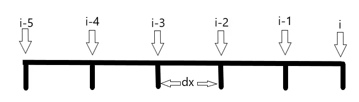
Let the hypothesis function be

`(del^2f)/(delx^2) = (a*f(i-5)+b*f(i-4)+c*f(i-3)+d*f(i-2)+e*f(i-1)+h*f(i))`

Using the taylor's table, the coefficients can be computed as shown below

Coefficients	f(i)	`Deltax f'(i)`	`Deltax^2f''(i)`	`Deltax^3f'''(i)`	`Deltax^4.f^(IV)(i)`	`Deltax^5f^(V)(i)`	`Deltax^6f^(VI)(i)`
a.f(i-5)	a	-5*a	(25/2)*a	-(125/6)*a	(625/24)*a	-(3125/120)*a	(15625/720)*a
b.f(i-4)	b	-4*b	(16/2)*b/2	-(64/6)*b	(256/24)*b	-(1024/120)*b	(4096/720)*b
c.f(i-3)	c	-3*c	(9/2)*c	-(27/6)*c	(81/24)*c	-(243/120)*c	(729/720)*c
d.f(i-2)	d	-2*d	(4/2)*d	-(8/6)*d	(16/24)*d	-(32/120)*d	(64/720)*d
e.f(i-1)	e	-e	(1/2)*e	-(1/6)*e	(1/24)*e	-(1/120)*e	(1/720)*e
h.f(i)	h	0	0	0	0	0	0
Sum	0	0	1	0	0	?	?

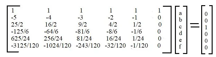
`he sum of the `Deltax^2f''(i)` is equal to one, and the rest of the sums are zero until the 5th order. The sums of the last two are unknown. Considering the terms until 5th order, we have 6 equations with 6 unknowns`

1. a+b+c+d+e+h = 0

2. 0-e-2d-3c-4b-5a= 0

3. 0+e/2+2d+(9/2)c+(16/2)b+(25/2)a = 1

4. 0 - e/6 - (4/3)*d - (27/6)*c - (64/6)*b - (125/6)*a = 0

5. 0 + e/24 + (16/24)*d + (81/24)*c + (256/24)*b + (625/24)*a = 0

6. 0 - e/120 - (32/120)*d - (243/120)*c - (1024/120)*b - (3125/120)*a =0

These equations can be converted into a matrix form, and solved in Matlab to find the 6 coefficients.

By solving the equations, we get

a = -0.8333

b = 5.0833

c = -13.0000

d = 17.8333

e = -12.8333

h = 3.7500

Using these values in the equations above in 1-6, the sum of equation 3 is 1, and the sum of the rest are zero.

Also, applying these coefficients to the sixth order coefficients, the sum of 6th order coefficients is non zero.

Therefore, the equation can be rewritten as

`(∂^2 f)/(∂x^2) = (a*f(i-5)+b*f(i-4)+c*f(i-3)+d*f(i-2)+e*f(i-1)+g*f(i))≅∆x^2 f''(x)+∆x^6 f^6(x)(CONSTANT)`

Dividing by `Deltax^2`we have

`(∂^2 f)/(∂x^2) = (a*f(i-5)+b*f(i-4)+c*f(i-3)+d*f(i-2)+e*f(i-1)+g*f(i))/(∆x^2)≅f''(x)+∆x^4 f^6(x)(CONSTANT)`

Here we can see, that the error term is of order 4. This is therefore, a fourth order approximation scheme.

A matlab script can be written to evaluate the three different approximation schemes

clear all
close all
clc

%Taylor table coefficients - central difference

A = [ 1 1 1 1 1;
    -2 -1 0 1 2;
    2 1/2 0 1/2 2;
    -8/6 -1/6  0 1/6 8/6;
    16/24 1/24 0 1/24 16/24];

B = [0;0;1;0;0];

X = A\B;

%Taylor table coefficients - skewed right hand scheme

C = [1 1 1 1 1 1;
    0 1 2 3 4 5;
    0 1/2 2 9/2 8 25/2;
    0 1/6 4/3 9/2 32/3 125/6;
    0 1/24 2/3 27/8 32/3 625/24
    0 1/120 32/120 243/120 1024/120 3125/120];

D = [0;0;1;0;0;0];

Y = C\D;


% Taylor table coefficients - skewed left hand scheme

E = [1 1 1 1 1 1;
    -5 -4 -3 -2 -1 0;
    25/2 16/2 9/2 4/2 1/2 0;
    -125/6 -64/6 -27/6 -8/6 -1/6 0;
    625/24 256/24 81/24 16/24 1/24 0
    -3125/120 -1024/120 -243/120 -32/120 -1/120 0];

F = [0;0;1;0;0;0];

Z = E\F;


%analytical function = exp(x)*cos(x)

x = pi/3;
dx = linspace(pi/4,pi/4000,300);

%analytical second derivative
analytical_derivative = -2*(exp(x))*(sin(x));

for i = 1:length(dx)
    error_central_diff(i)=central_diff(x,dx(i),X);
    error_left_diff(i)=left_diff(x,dx(i),Z);
    error_right_diff(i)=right_diff(x,dx(i),Y);
end

figure(1)
loglog(dx,error_central_diff,'g','linewidth',2);
hold on
loglog(dx,error_left_diff,'r','linewidth',2);
hold on
loglog(dx,error_right_diff,'y','linewidth',2);

xlabel('dx');
ylabel('error');
title('Dx (grid size) vs Error');
legend('Central diff error','Left diff error','Right diff error');

The functions for the three approximation schemes are shown below

1. Central difference

function out = central_diff(x,dx,X)

%analytical function = exp(x)*cos(x)

%analytical second derivative
analytical_derivative = -2*(exp(x))*(sin(x));

%Central difference scheme
central_diff = ((X(1)*exp(x-(2*dx))*cos(x-(2*dx))) + (X(2)*exp(x-(1*dx))*cos(x-(1*dx)))+(X(3)*exp(x)*cos(x))+(X(4)*exp(x+(1*dx))*cos(x+(1*dx)))+ (X(5)*exp(x+(2*dx))*cos(x+(2*dx))))/(dx^2);

% Errors
out = abs(central_diff - analytical_derivative);

end

2. Skewed right difference

function out = right_diff(x,dx,Y)

%analytical function = exp(x)*cos(x)

%analytical second derivative
analytical_derivative = -2*(exp(x))*(sin(x));

%Right difference scheme
right_diff = ((Y(6)*exp(x+(5*dx))*cos(x+(5*dx))) + (Y(5)*exp(x+(4*dx))*cos(x+(4*dx)))+(Y(4)*exp(x+(3*dx))*cos(x+(3*dx)))+(Y(3)*exp(x+(2*dx))*cos(x+(2*dx)))+ (Y(2)*exp(x+(1*dx))*cos(x +(1*dx)))+ (Y(1)*exp(x)*cos(x)))/(dx^2);

% Errors
out = abs(right_diff - analytical_derivative);

end

3. Skewed left difference

function out = left_diff(x,dx,Z)

%analytical function = exp(x)*cos(x)

%analytical second derivative
analytical_derivative = -2*(exp(x))*(sin(x));

%Left difference scheme
left_diff = ((Z(1)*exp(x-(5*dx))*cos(x-(5*dx))) + (Z(2)*exp(x-(4*dx))*cos(x-(4*dx)))+(Z(3)*exp(x-(3*dx))*cos(x-(3*dx)))+(Z(4)*exp(x-(2*dx))*cos(x-(2*dx)))+ (Z(5)*exp(x-(1*dx))*cos(x -(1*dx)))+ (Z(6)*exp(x)*cos(x)))/(dx^2);

% Errors
out = abs(left_diff - analytical_derivative);

end

Results

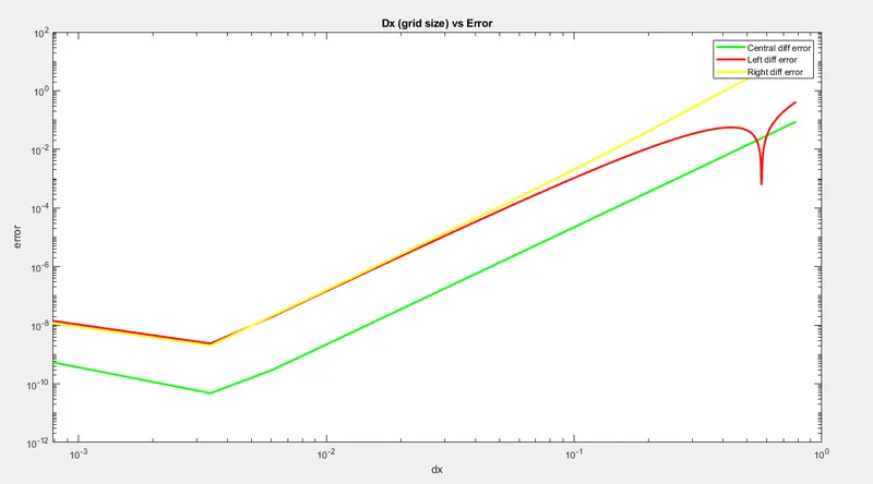
The errors of the three approximation schemes are plotted in a log plot, as shown below

Observations

The central difference scheme has a lower starting error, and the error reduces until a certain value of dx, and then increases slightly.

This trend is seen in the other two approximation schemes as well, but their errors and the convergence rates are slightly higher.

The minimum error in all three schemes can be seen below

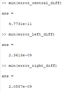
It can be seen, that the central difference scheme is the most accurate, and the skewed left and right difference schemes have almost a similiar degree of accuracy.

Conclusion

Thus , the fourth order approximation of the second derivative of the function has been approximated numerically using the different schemes, and the results have been illustrated for comparison of the errors.

The related matlab m files have been attached below.