Week-6 Calculate the Stretch Ratio by comparing the ELFORM (-2,-1,1,2) with Ogden_Material Model.
Objective:
To simulate the tensile behaviour of a solid block with different element formulations and compare the stretch ratios from each case.
Step 1: Solid block creation and section definition
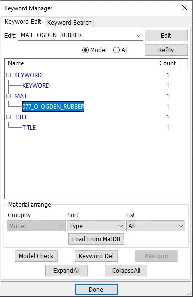
The given keyword file, which contains the Ogden Material definition is opened in LS Dyna. The default values of the hyperelastic material definition can be retained.
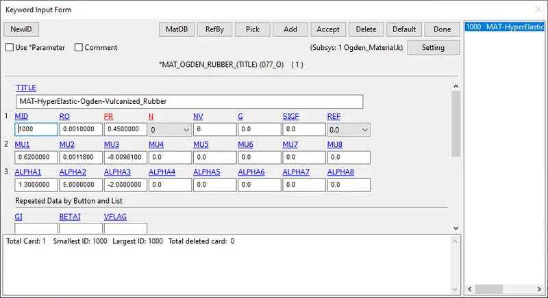
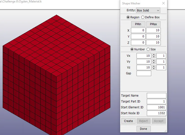
A FE model of a solid box is created using Shape mesher option under Element and Mesh panel as shown below.
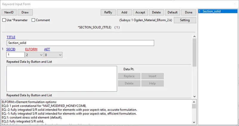
Section definition
The section properties for the solid block are assigned as shown below. The different element formulations, that need to be tested are ELFORM 1,2, -1 and -2.
Part Definition
The material and the section are then assigned to the part ID of the solid block as shown below.
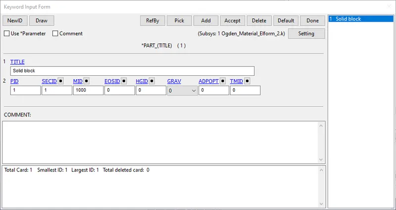
The definitions with different ELFORMS are saved separately in a keyword file and simulated individually to obtain the results.
Step 2: Boundary conditions
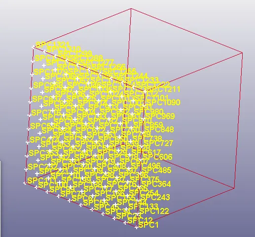
SPC - X direction
The nodes of the box on the YZ plane are selected and their motion is constrained in the X-direction, since they should be fixed.
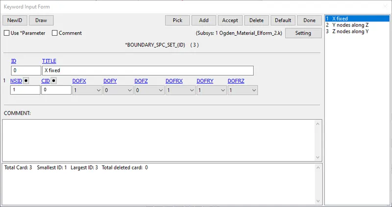
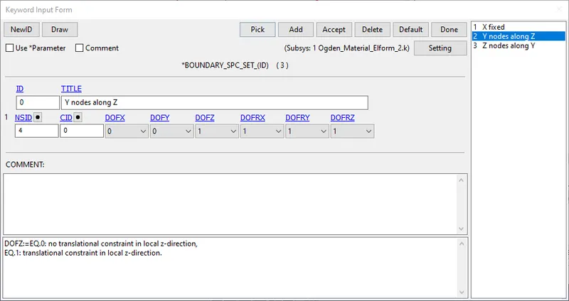
SPC - Z Direction
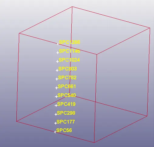
The motion of the middle nodes in the Y direction is constrained in the Z - direction, to avoid vertical displacement.
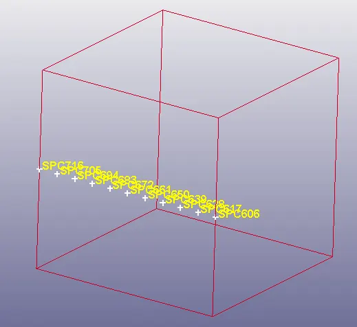
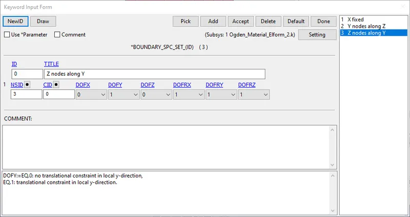
SPC - Y Direction
The motion of the middle nodes in the Z direction is constrained in the Y - direction, to avoid lateral displacement.
Prescribed motion
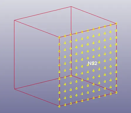
The nodes on the opposite side of the YZ plane are selected and a displacement is given to them according to the minimum load to be applied on the moving surface to achieve a stretch ratio of 5, as shown below.
Engineering strain `epsilon_e = (deltal)/ l`
Stretch ratio `lambda = 1 + epsilon_e`
`5 = 1 + (deltal)/10`
`deltal = 40 mm`
Therefore, a minimum value of 50 mm is taken to define the load curve.
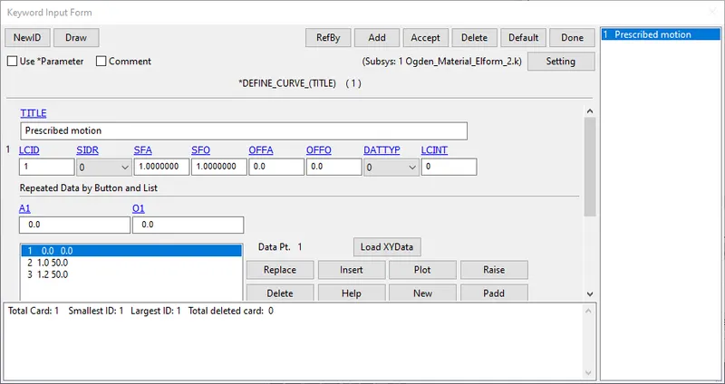
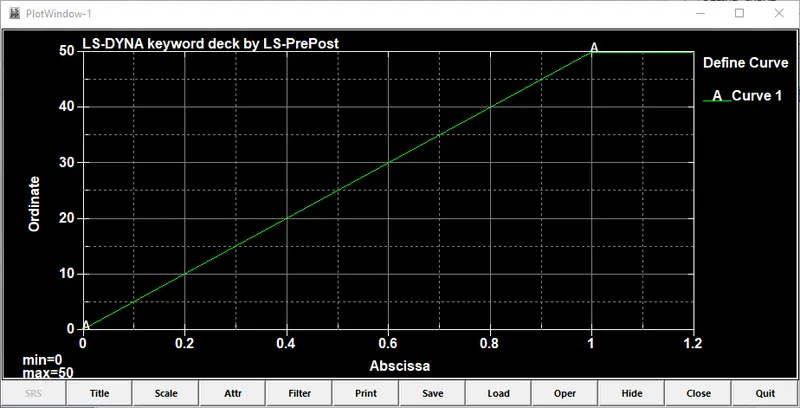
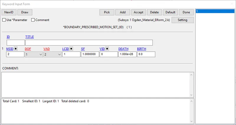
The above shown load curve is assigned to the nodes using the appropriate LCID as shown below.
Step 3: Control cards
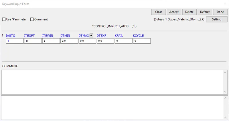
A control_implicit_auto card, with IAUTO set to 1, is used for automatic timestep adjustment.
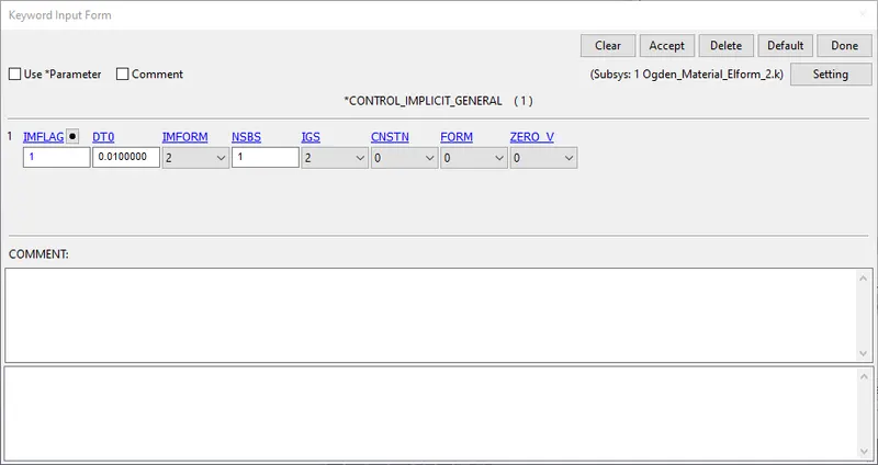
A control_implicit_general card is used with IMFLAG = 1 to specify that an implicit solving scheme needs to be used. The initial timestep value DT0 is set to 0.01.
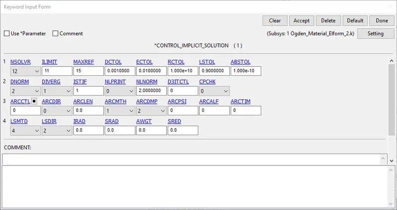
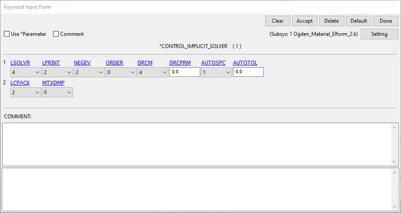
A control_implicit_solution card is used to specify whether a linear or a non linear solution is desired. This card is used with default parameters.
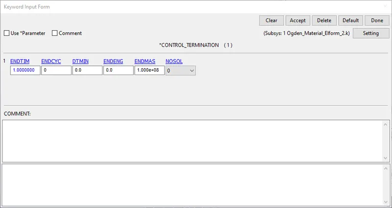
The simulation time is set as 1 ms using the control_termination card.
Step 4: Database cards
A database_binary_D3 plot is defined with an output frequency DT of 0.01 ms.
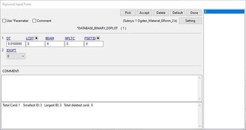
Under DATABASE_ASCII, GLSTAT and ELOUT are selected with the same value of DT.
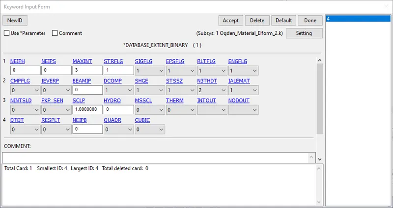
A DATABASE_EXTENT_BINARY card is used with STRFLG = 1, in order to compute the elastic strain in the model.
The keyword file is checked for errors using the Model Checker and saved before starting the simulation.
Results
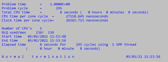
The simulation is completed with the following message showing a NORMAL TERMINATION
X-Stress
The uniaxial stress plots of the 4 cases can be plotted as shown below and the maximum stress in the X-direction can be visualized.
ELFORM 1

ELFORM 2
ELFORM -1
ELFORM -2
The peak stresses are as follows
ELFORM 1 - 5.024 MPA
ELFORM 2 - 5.031 MPA
ELFORM -1 - 5.024 MPA
ELFORM -2 - 5.024 MPA
X-Strain
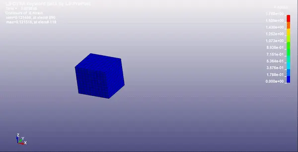
The uniaxial strain plots of the 4 cases can be plotted as shown below and the maximum strain in the X-direction can be visualized.
ELFORM 1
ELFORM 2
ELFORM -1
ELFORM -2
The peak strains are as follows
ELFORM 1 - 1.788
ELFORM 2 - 1.789
ELFORM -1 - 1.788
ELFORM -2 - 1.789
Calculation of engineering strain, engineering stress and stretch ratio
The output of the D3 plot in LS Dyna gives true stress and true strain. The engineering stress and strain can be calculated using the relations below.
True stress `sigma_t = sigma_e (1 + epsilon_e)`
Engineering stress `sigma_e = sigma_t / (1 + epsilon_e)`
True strain `epsilon_t = ln(1 + epsilon_e)`
Engineering strain `epsilon_e = e^(epsilon_t) - 1`
Stretch ratio `lambda = 1 + epsilon_e`
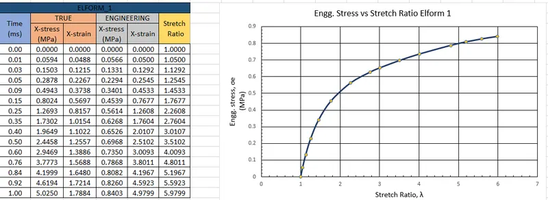
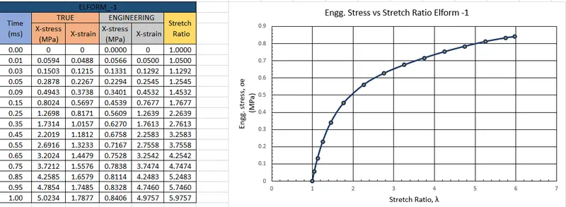
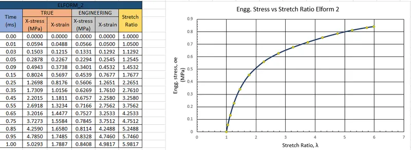
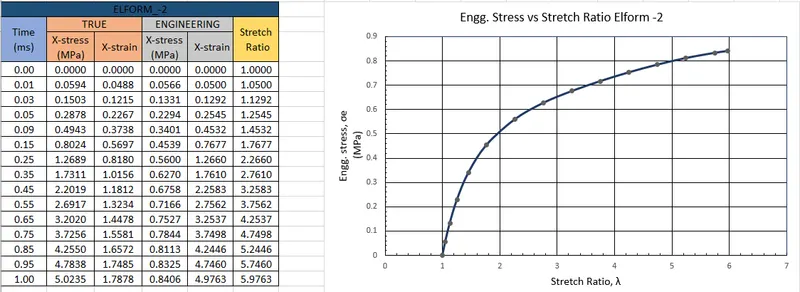
The values of the true stress and strain are imported into an excel sheet and the computation of the engineering stress and strain for the 4 cases are done as shown below. The plot of Engineering stress against the stretch ratio for each case is also shown for each case.
ELFORM 1
ELFORM -1
ELFORM 2
ELFORM -2
Comparison
From the graphs of Engineering stress vs stretch ratio, the max value at a stretch ratio of 5 is approximately 0.8 MPA.
The values from the 4 cases are almost the same, due to the simplicity of the model considered.
Conclusion
Thus the FE model of a solid block has been simulated for uniaxial loading with various element formulations and the results of engineering stress vs stretch ratio have been compared.
The related files and the excel sheet can be found under the link below
https://drive.google.com/drive/folders/1VcNRCMKQZD39_S_S-NxXt7R7kqpP-qUd?usp=sharing