Week 6: Conjugate Heat Transfer Simulation
Objective
To simulate the conjugate heat transfer flow with various grid sizes and super cycle time values and illustrate the results.
Theory
CHT Analysis
Conjugate heat transfer (CHT) analysis can accurate predict heat transfer by simultaneously solving all the relevant solid and flow field heat transfer processes, for example condution through solids, free and forced convection in the gases/ fluids and thermal radiation.
Conjugate heat transfer corresponds with the combination of heat transfer in solids and heat transfer in fluids. In solids, conduction often dominates whereas in fluids convection usually dominates. Efficiently combining heat transfer of fluids and solids is the key to designing effective coolers, heaters or heat exchangers. Forced convection is the most common way to achieve high heat transfer rate. In some applications, the performances are further improved by combining convection with phase change.
Supercycling
We have the simulation through two different mediums - fluid and solid. This leads to the simulations through the mediums at different speeds - faster through the fluid and slower through the solid. The fundamental idea of super cycle modeling is that the fluid simulation is held until the solid simulation converges at each time step. This ensure consistency and leads to simulation without global convergence issues.
Y+
The Y+ criteria is important to capture the physics near the solid wall boundary. The Y+ criteria determines the fineness or coarseness of the mesh near the wall boundary. For turbulent flows, the laminar region is very small and a very small grid size is needed to get accurate results. If y+ is in the range of 0-10, we can capture laminar flow and for values higher than 30 we capture turbulent flow.
Solution
Geometry creation
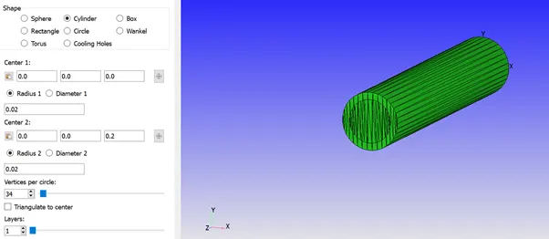
Two concentric cylinders with radii 0.015m and 0.02m are created, and the side faces are removed to represent the pipe.
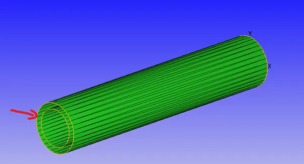
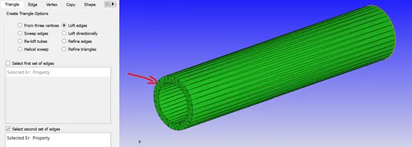
The side thickness is sealed on both sides, to represent a solid portion. This is done using the Triangle loft option under Create
The boundaries are flagged for the outer surface and the side walls. The patch option is used to seal the inlet and the outlet sides. The inside face of the cylinder is the interface between the solid and the fluid regions.
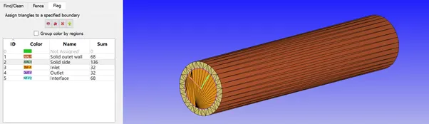
The diagnosis tool shows the presence of non-manifold edges, due to the inlet and outlet edges being shared by three surfaces. This is normally the case in a CHT problem, and this is resolved automatically, when the case is setup for simulation.
Case Setup
A time based simulation is selected with the material as Air.
The values for the global transport parameters and reaction mechanism is disabled.
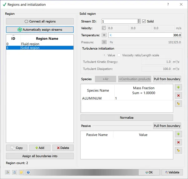
Both gas and solid simulation are used, with Aluminium as the solid material.
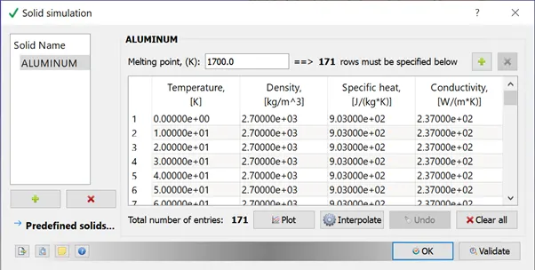
The values of the global transport parameters are kept constant, and under Species o2 and N2 are used for gas, and Aluminium for solid.
Simulation parameters
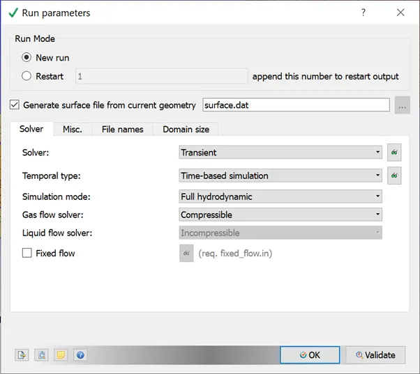
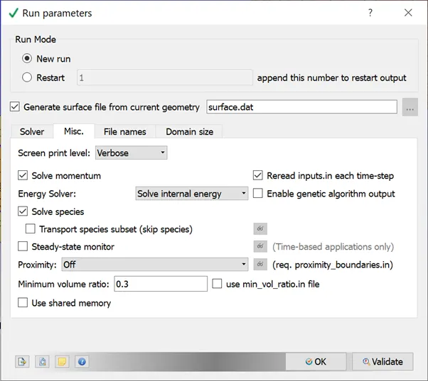
A transient, full hydrodynamic compressible solver is selected as shown below. The steady state monitor is turned off, and the use of shared memory is unchecked.
An end time of 0.5s is used, with an initial and minimum time step of 1e-7s.
The maximum time step is given as 1s.
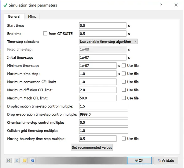
The solver parameters are kept default.
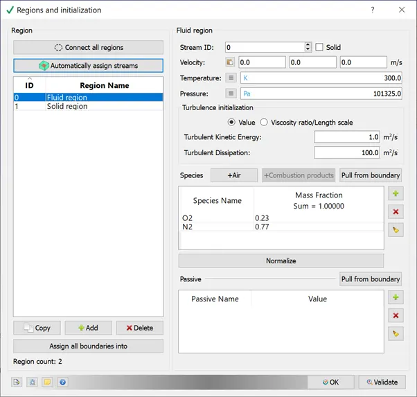
The regions are initialized as follows
Region 0 is the fluid region, and the flow fluid here is air.
Region 1 is the solid region made of aluminium. The Stream ID has to be selected as 1.
Boundary conditions
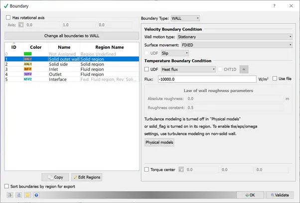
Solid outer wall
Since this is stationary, it is modelled as a fixed wall with a heat flux of -10000 W/m^2.
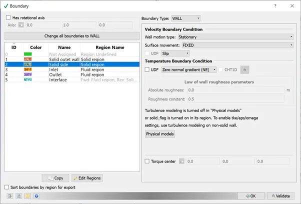
Sides
The sides are modelled as Slip walls with Neumann boundary condition for Temperature.
Inlet
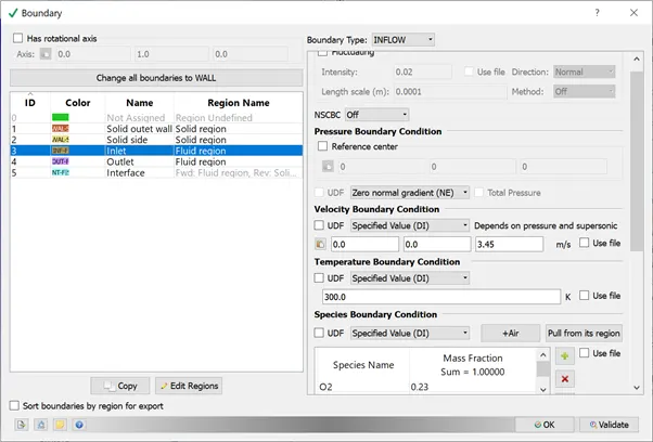
The pressure at the inlet is given using a Neumann boundary condition, and values are given for temperature and velocity.
The flow velocity is calculated using the given Reynold's number of 7000. The inner diameter is 0.03m. The values of density and viscosity are mentioned below.
`Re=(rho*V*D)/mu, where" "rho=1.225kg"/"m^3,D=0.03m,mu=1.85e"-"05kg"/"ms`
`V=(7000"*"1.85e"-"05)/(1.225"*"0.03)=3.45m"/"s`
Outlet
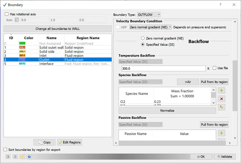
The outlet is modelled with Dirichlet BC for velocity and Air as the species for backflow.
Interface
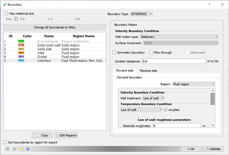
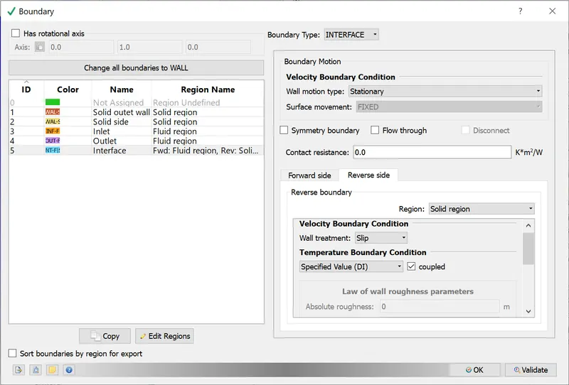
The interface is in contact with both the solid and the fluid region. Therefore it has to be defined on the forward and the reverse sides.
Forward side
The forward side is the fluid region with law of wall for velocity and temperature BCs.
Reverse side
The reverse side is the solid region with slip wall for velocity and dirichlet condition for temperature.
Physical models
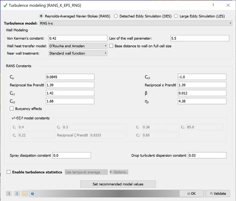
The K EPSILON model with default parameters is used for modeling turbulence.
Super cycle modeling
Super cycle modeling is turned on.
The super cycle data parameter is chosen as 0.05 for the baseline grid size (0.004m).
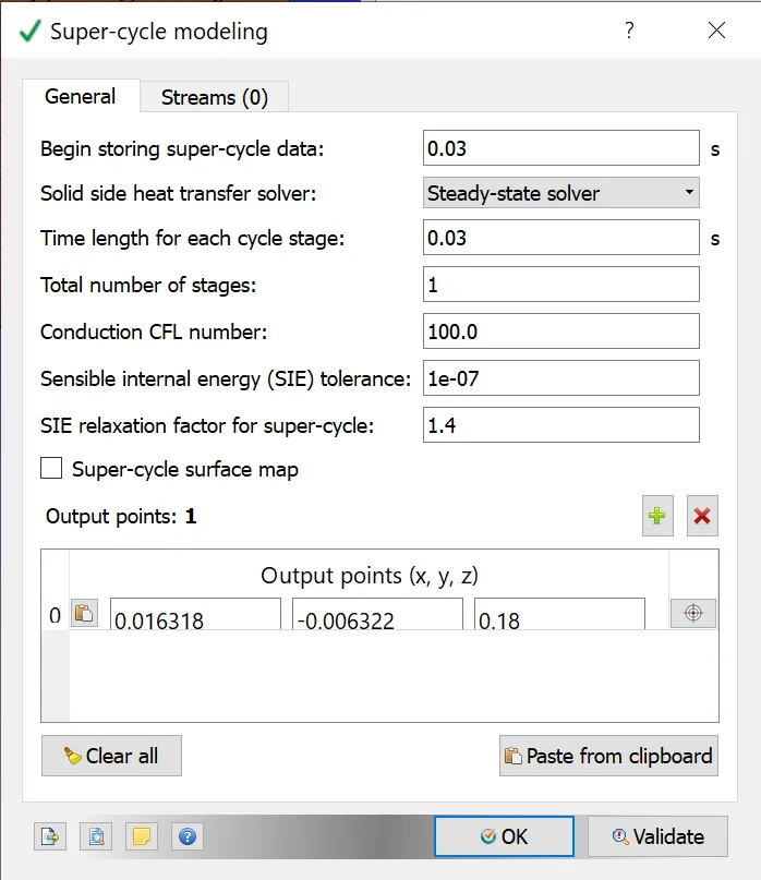
The output point has to be chosen within the boundary of the model, such that the temperature changes are captured. The co-ordinates of this point can be calculated with the help of the Measure --> Average of vertex locations option.
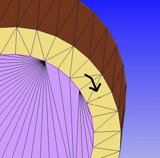
The baseline grid size is 0.004m as mentioned above.
The 3d output files are written every 0.01 seconds and the time interval for the text output is 1e-6 s.
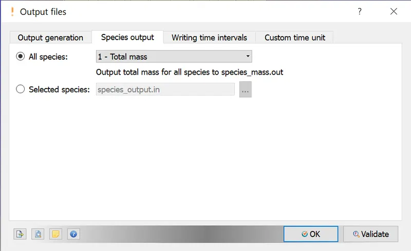
Under post variable selection, y+ variable is checked under turbulence parameters.
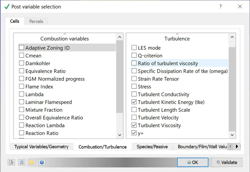
The model is setup for simulation and the results can be viewed in the line plotting tool and in Paraview.
The simulation is carried out for three different grid sizes
1. 0.004 m
2. 0.003 m
3. 0.002 m
Results
Grid size -0.004m
Mesh
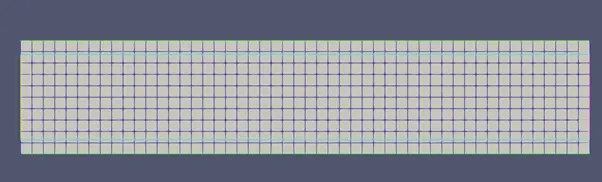
Velocity contour
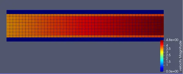
The inlet velocity is 3.45 m/s. As the air passes through the tube, the velocity increases due to lower static pressure, and the value at the output is 4.8 m/s.
Temperature contour
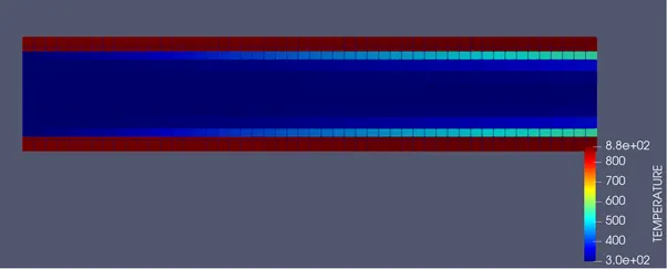
The outer wall is around 880 degree celsius and the temperature of the air (fluid) at the outlet is around 360 degree celsius.
Pressure contour
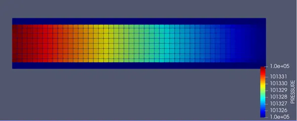
The inlet is defined with Neumann BC. The pressure at the inlet is 1 bar and at the outlet it is almost the same, with a slightly lower value.
Y+
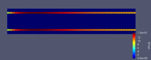
The peak Y+ value here is 15, which means that the flow is in the transition phase. It has minor significance for CHT modeling.
Grid size - 0.003m
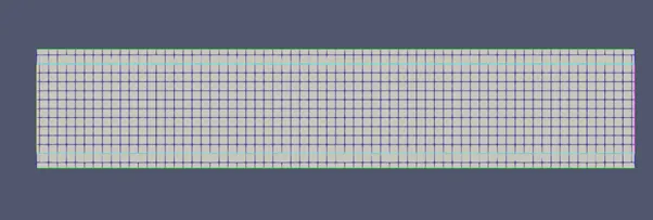
Mesh
Velocity contour
The inlet velocity is 3.45 m/s. As the air passes through the tube, the velocity increases due to lower static pressure, and the value at the output is 4.9 m/s. 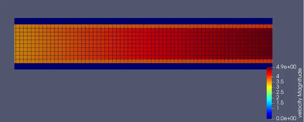
Temperature contour
The outer wall is around 850 degree celsius and the temperature of the air (fluid) at the outlet is around 350 degree celsius. 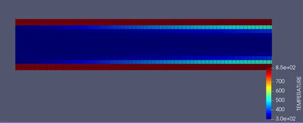
Pressure contour
The inlet is defined with Neumann BC. The pressure at the inlet is 1 bar and at the outlet it is almost the same, with a slightly lower value.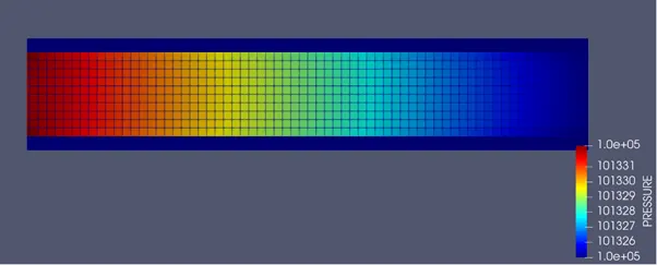
Y+
The peak Y+ value here is 15, which means that the flow is in the transition phase. It has minor significance for CHT modeling.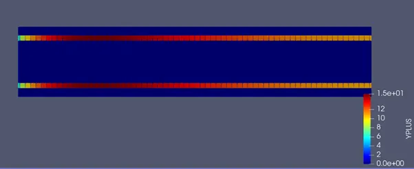
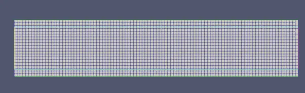
Grid size - 0.002m
Mesh
Velocity contour
The inlet velocity is 3.45 m/s. As the air passes through the tube, the velocity increases due to lower static pressure, and the value at the output is 5.1 m/s. 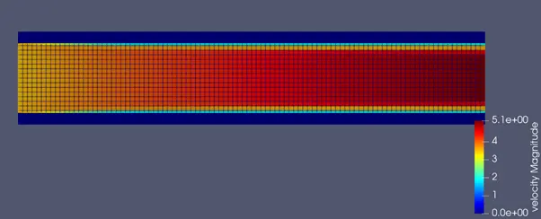
Temperature contour
The outer wall is around 770 degree celsius and the temperature of the air (fluid) at the outlet is around 350 degree celsius. 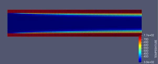
Pressure contour
The inlet is defined with Neumann BC. The pressure at the inlet is 1 bar and at the outlet it is almost the same, with a slightly lower value.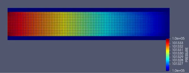
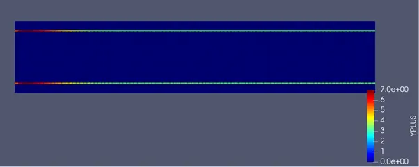
Y+
The peak Y+ value here is 7, which means that the flow is in the laminar phase. The physics of the flow can be captured well.
Comparison
Grid dependence test
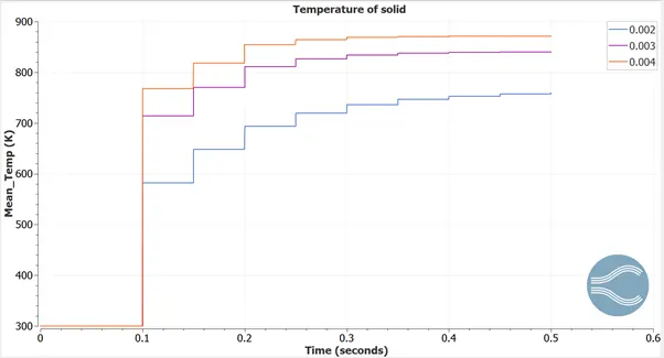
Temperature solid
Inferences
The mean temperature follows a step like curve as super cycling is enabled.
The accuracy of temperature increases as the mesh or the grid size is reduced.
The temperature converges to 880K, 850K and 770K for mesh sizes of 4mm, 3mm and 2mm respectively.
This means that the value of temperature is very dependent on the grid size and it varies drastically.
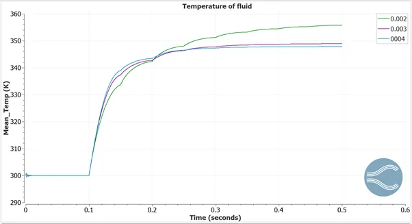
Temperature fluid
Inferences
The above figure shows the variation of temperature of the fluid with time.
The mean temperatures converge to values of 360 K, 350K and 350K for mesh sizes of 4mm, 3mm and 2mm respectively.
In spite of different mesh sizes, the final temperature value for the 3mm and 4mm mesh are the same.
Number of cells
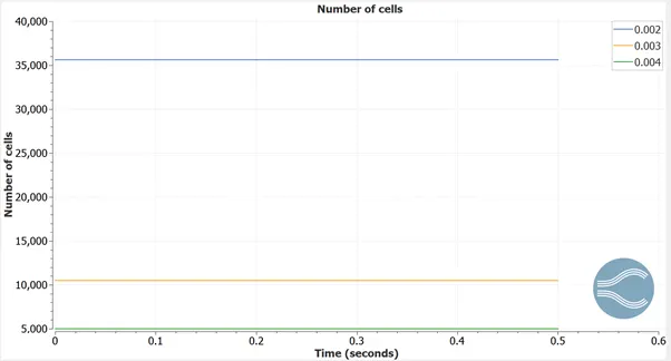
The important results can be summarized in the table below

Inferences
As the number of cells is higher for mesh size of 2mm, the results are highly accurate, because the physics of the problem are captured better.
Supercycle stage
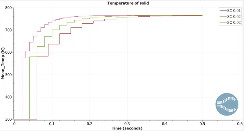
Temperature plot for solid
Temperature plot for fluid
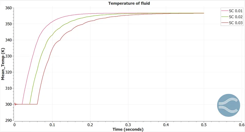
Inferences
The above plots show the effect of super cycling time on the temperature of the solid and the fluid mediums.
As the time length is reduced, the solution converges at a faster rate and reaches the steady state value faster.
The mean temperature for the solid and fluid converge to 770 K and 358 K respectively much faster with an SC of 0.01. As the time interval is increased, the time taken to reach the steady state increases.
The important results can be summarized in the table below

Inferences
The simulation run time increases, as the super cycle stage is increased, since the time taken to attain steady state increases.
The number of cycles is inversely proportional to the increase of the super cycle stage.
Conclusion
Thus, the simulation of conjugate heat transfer through a pipe has been performed, and the results of the grid dependence test and the super cycle grade have been illustrated.
Animation pressure - Grid size 0.002, SG: 0.05
Animation velocity - Grid size 0.002, SG: 0.05
Animation y+ - Grid size 0.002, SG: 0.05