Week 10: Modeling and Simulation of flow around an Ahmed Body
Objective
To simulate the flow around an Ahmed body using converge CFD and compare the simulation results with the experimental data.
Theory
The ahmed body is a generic car body, which can be used to predict first aerodynamic simulation results. The airflow around the Ahmed body captures the essential flow features around an automobile and was first defined and characterized in the experimental work of Ahmed. Although it has a very simple shape, the Ahmed body allows us to capture characteristic features that are relevant to bodies in the automobile industry.
The model's dimensions are 1044mm x 389mm x 288mm
The specific angle at the rear is 35 degrees.
Solution
The boundary layer thickness is 30 mm at 400 mm in front of the Ahmed body
`delta=frac{0.382*x}{Re^2}`
where `delta`is the boundary layer thickness.
x = length of the plate (m)
Re = Reynolds number
`0.03=frac{0.382*x}{frac{rhoVx}{mu}^2}`
`(x)^0.8=(0.03)* frac{frac{1.225*40}{1.85*10^-5}}{0.382}`
x = 1.66m
Therefore, 1.66m in front of the Ahmed body, the boundary layer thickness is 30 mm.
The actual no slip region in front of the ahmed body is 1.66+0.4 = 2.04 m
Therefore the slip region can be taken as 2m. the region behind the Ahmed body until the Outflow is 5*L, where L is the length of the Ahmed body. 5*1.044 = 5.22 m
Geometry creation - Solidworks
The Ahmed body is created in solidworks according to the dimensions shown below
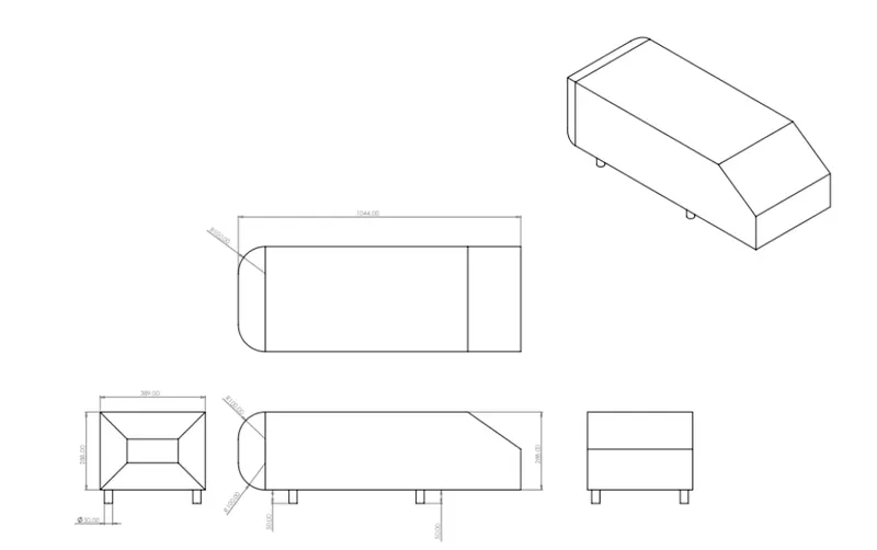
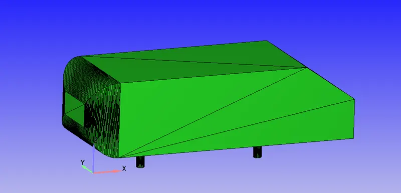
It can be imported as an STL file into Converge.
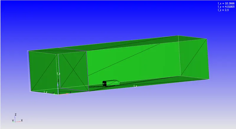
The next step is to calculate the virtual wind tunnel. Its dimensions are
X direction = 2.04 + 1.044 + 5*22 = 8.264
A length of 2m is added to this. Therefore the total length is Dx = 10.264m
The other dimensions are Dy = 4m, Dz = 2.5m
The normals are transformed to point into the region of fluid flow.
Boundary creation
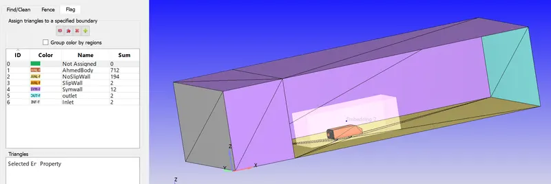
A total of 6 different boundaries were created as shown below.
Case setup
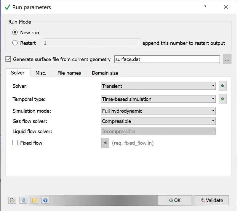
A time based simulation is selected with Gas simulation and Air as the predefined mixture.
The default values are used for the global transport parameters.
Simulation parameters
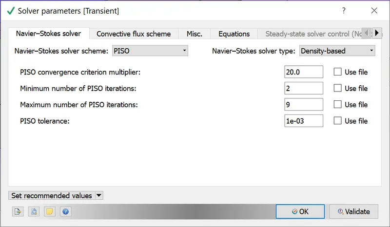
A transient, density based, PISO solver is selected.
Calculation of time
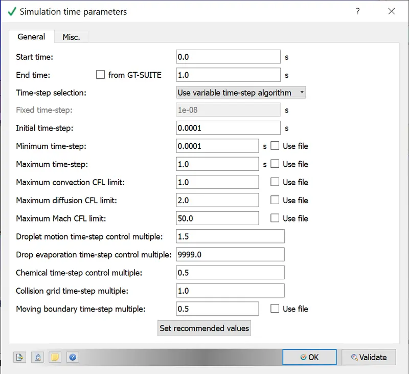
Length = 10.264m
Average velocity (given) = 40m/s
Speed = Distance/time
Therefore time = 0.256 s
We are simulating roughly 4 times of flow - 1 s
Boundary conditions
The boundary conditions for each boundary are defined as follows
| S.No | Boundary_name | Boundary_type | Value | Boundary ID |
| 1 | Ahmed body | Wall | Law of wall | 1 |
| 2 | No Slip wall | Wall | Law of wall | 2 |
| 3 | Slip wall | Wall | Slip wall | 3 |
| 4 | Symmwall | Symmetry | 4 | |
| 5 | Outlet | Outflow | 101325 Pa at 300 K (Dirichlet BC) | 5 |
| 6 | Inlet | Inflow |
Velocity - 40 m/s in X axis Pressure - neumann BC |
6 |
Initial conditions and Events
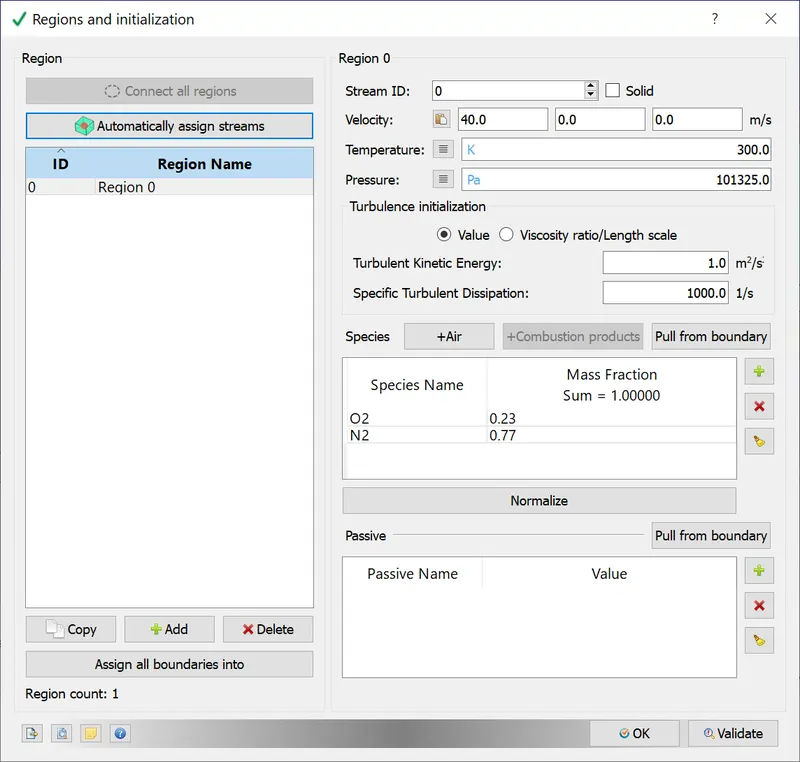
A volumetric regions was created in order to assign this to the boundary tags.
Species - O2 (0.23) and N2 (0.77)
Pressure - 101325 Pa
Temperature - 300K
Velocity - 40m/s - X axis
Physical models
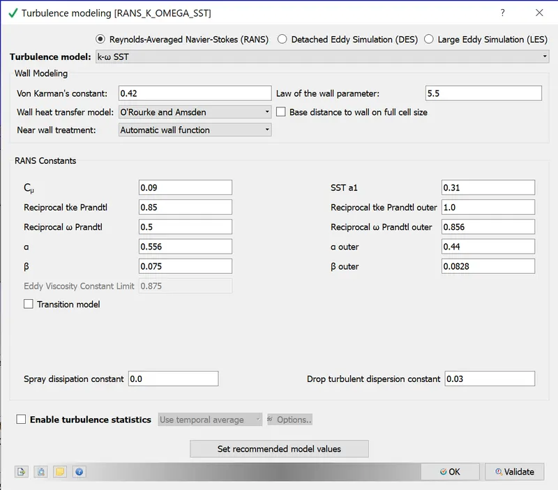
A K-omega-SST model is selected. It is a combination of the RNGl-E and standard K-omega model. Near the wall it works as a standard K-omega model and away from the wall, it works as a RNGk-Epsilon model. Hence it gives an accurate prediction near and away from the wall, since capturing the behaviour in the boundary layer is quite significant here.
Grid control
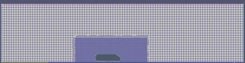
The mesh size is
dx - 0.1m, dy = 0.1m, dz - 0.1m
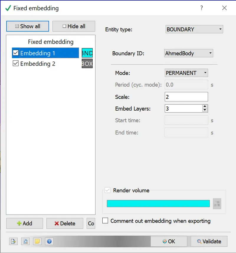
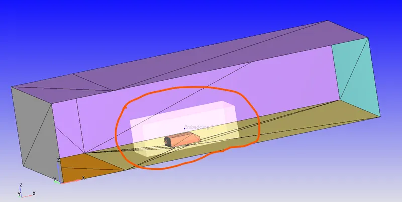
Fixed embedding is used in order to capture the edges of the Ahmed body better
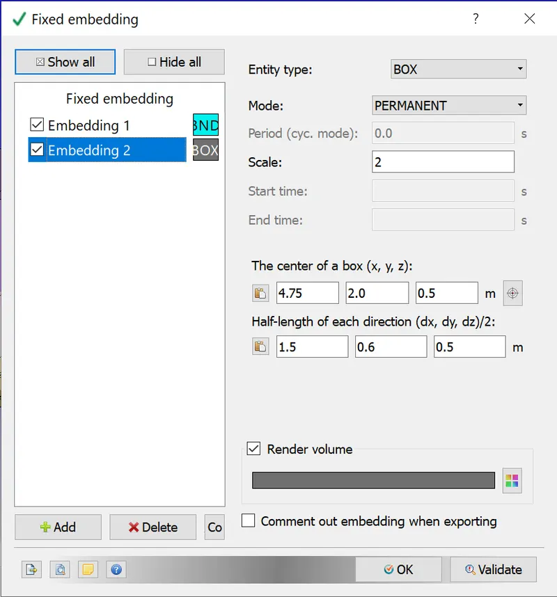
In addition, fixed embedding is applied to a specific volume surrounding the ahmed body, in order to capture the flow physics in this area better.
Output/Post processing
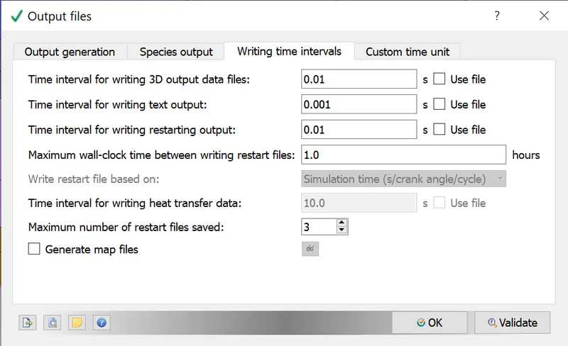
Time interval for writing the 3D output files - 0.01s
Time interval for writing restart files - 0.01s
The simulation was run using CYGWIN, and the post processing was done in ParaView.
Results
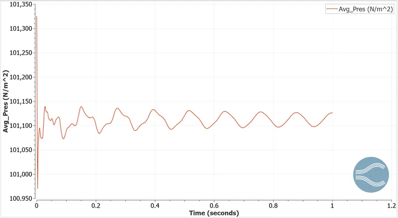
Pressure plot
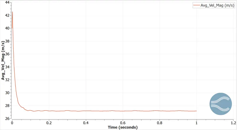
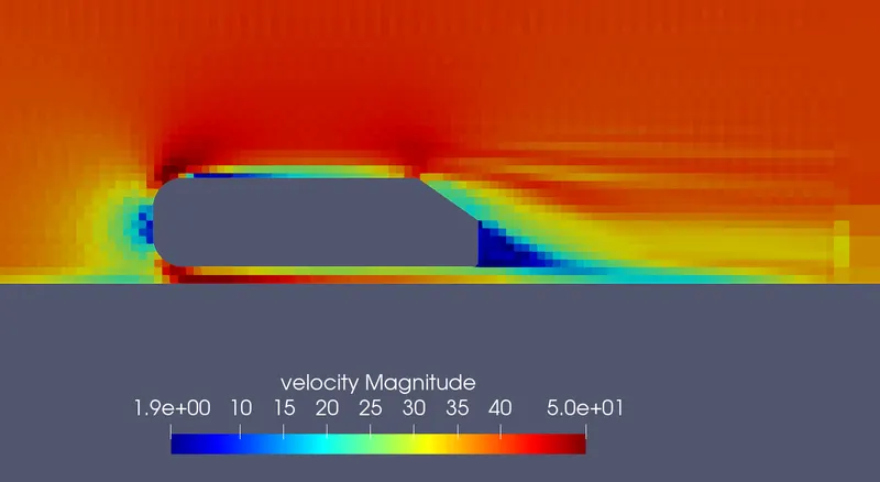
Velocity plot
Paraview
Mesh
Velocity contour
Slice plane
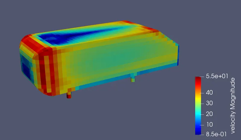
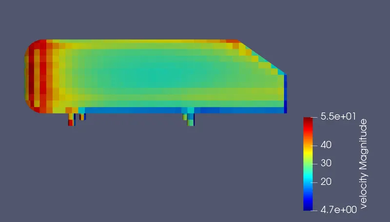
Extracted block - Ahmed body
Observation
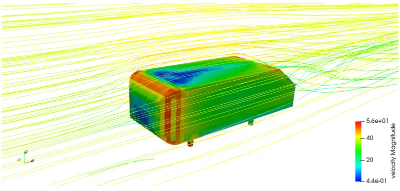
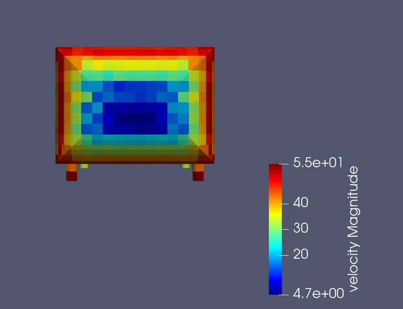
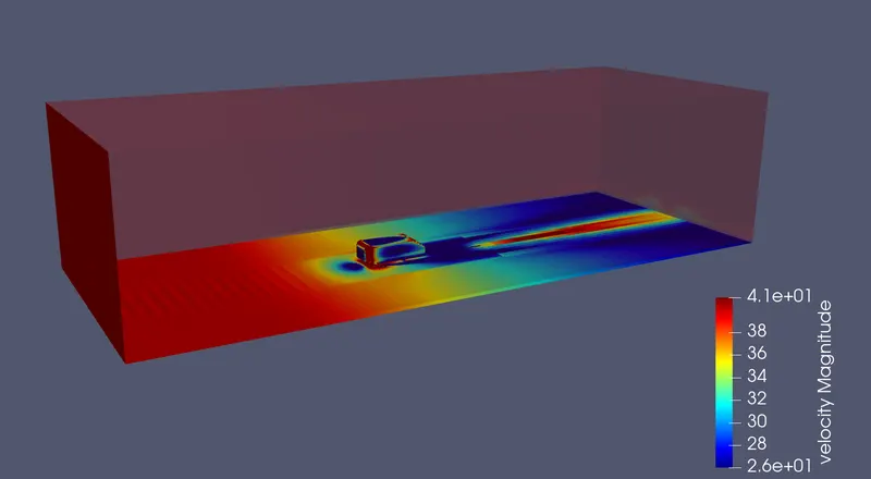
The velocity at the rear of the Ahmed body is very low, and there is a formation of recirculation zone. On the top and side surface of the Ahmed body, there is a layer of low velocity, since the flow does not stay attached to the body throughout. It reattaches, and separates again over the slant at the rear, which is another region of recirculation.
The air strikes the front area and loses its kinetic energy. The low velocity region along the trailing edge is called the wake region, which is due to the slant angle of the Ahmed body - 35 deg. This contributes to the majority of the drag forces on the body.
Pressure contour
Slice plane
Extracted block - Ahmed body
Observation
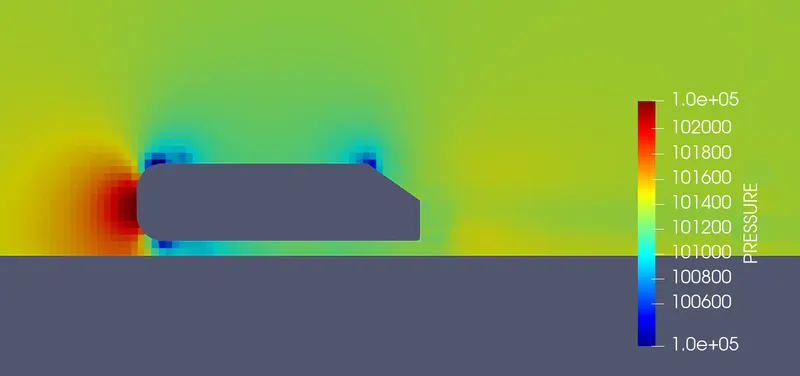
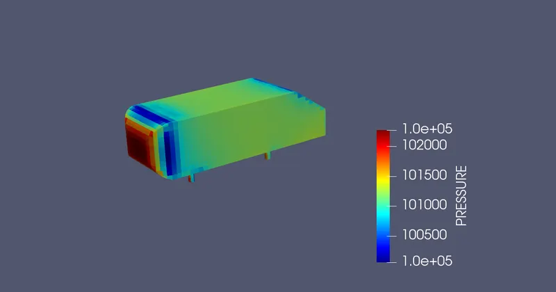
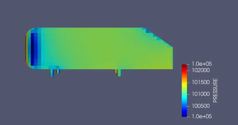
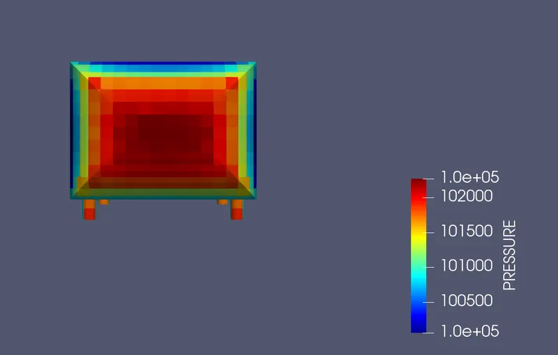
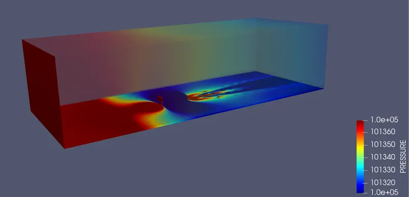
The pressure is very high on the front face of the Ahmed body. The flow stagnates here, as also illustrated in the velocity contour.
The pressure is very low at the front edges, as the flow flows over them and is accelerated due to the convexity of the edges.
Over the top and the side walls, the pressure is slightly higher, which corresponds with the low velocity flow, as the flow separates and reattaches towards the rear.
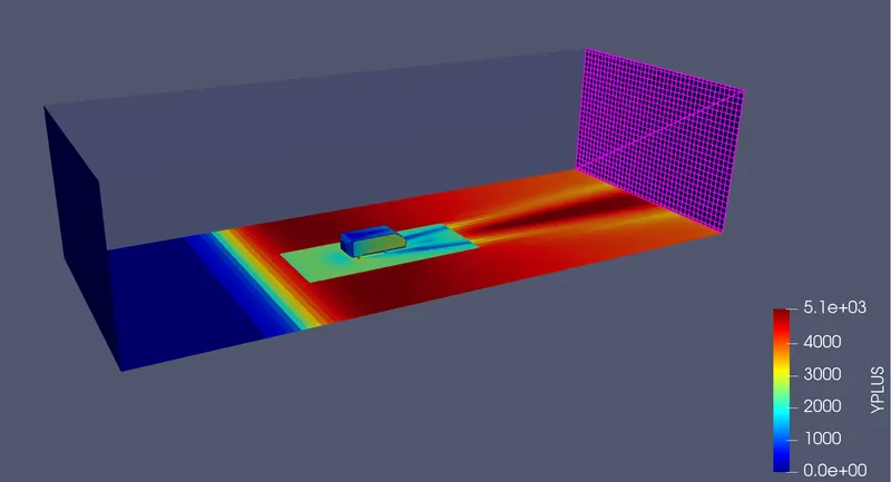
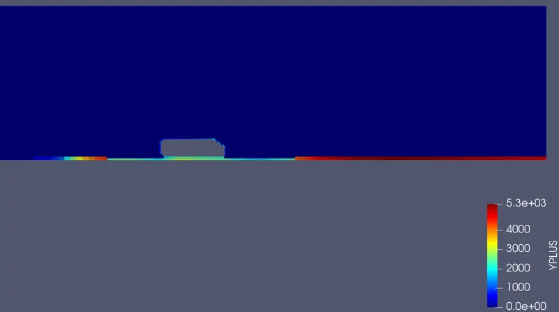
Y plus
Velocity at various points along the region
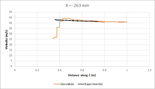
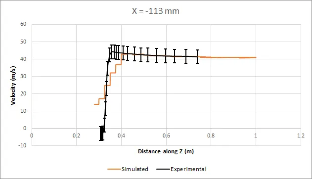
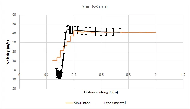
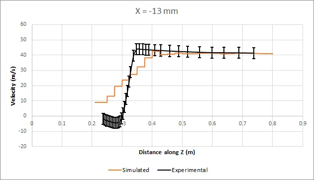
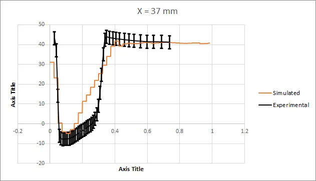
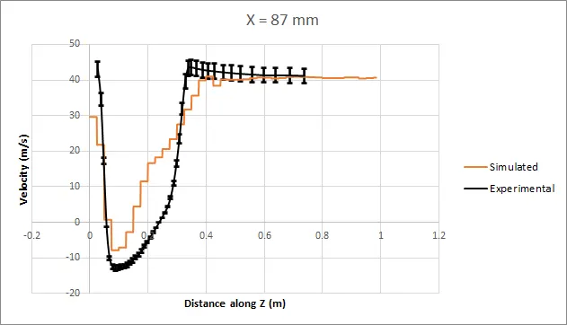
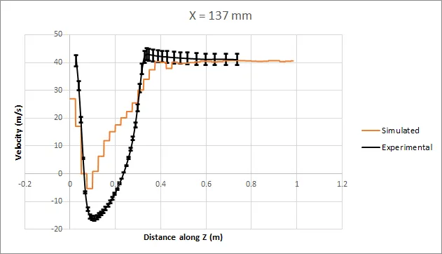
The simulated values of velocity are compared with the experimental values, in order to evaluate the accuracy of the results obtained.
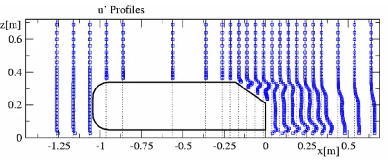
The back face of the Ahmed body is the origin point. The points to the left are negative X and those on the right are positive X.
X = -263 mm
X = -113 mm
X = -63 mm
X = -13 mm
X = 37 mm
X = 87 mm
X = 137 mm
X = 187 mm
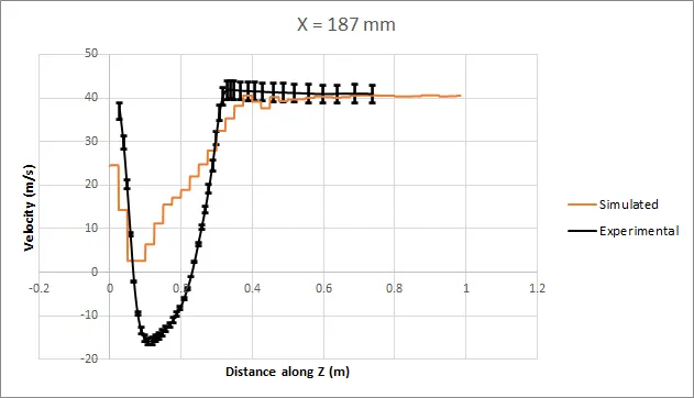
The plots show a reasonable convergence between the experimental and the simulated data. The error is due to the mesh size and the simplicity of the mesh, due to cost of computation.
Normalized velocity plot
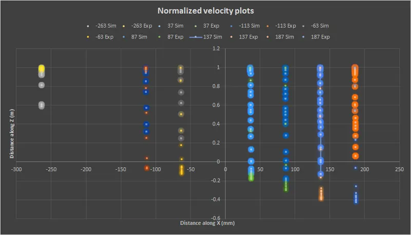
The normalized plots show a good correlation between experimental and simulated data at points forwards and rearwards of the back face of the Ahmed body.
The positive X points represent the region behind the Ahmed body where there is formation of a recirculation zone, that has low pressure and low velocity. When the probe is just below the Ahmed body, the velocity is high, then slowly it approaches the recirculation zone that has low pressure.
Calculation of lift and drag forces using Paraview (and correlated with Converge plots)
After the group files are imported into Paraview, the Ahmed body can be isolated using the Extract Block filter.
Next, the surface of the Ahmed body is extracted using Extract Surface filter.
The surface normals are then created using the corresponding filter.
The lift and drag forces can then be calculated using the Virtual calculator.
Lift force (single cell) = PRESSURE (scalar) * Normals_Z
Drag force (single cell) = PRESSURE (scalar) * Normals_X
The cell data is then integrated using a filter called "Integrable variable"
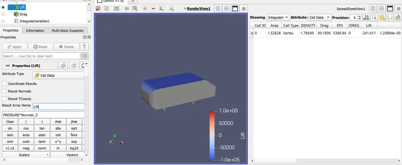
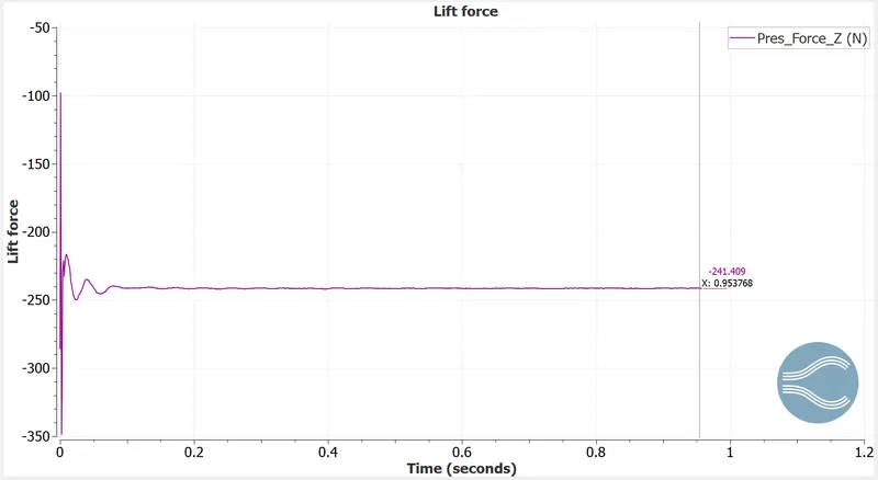
The lift force is -241.41 N.
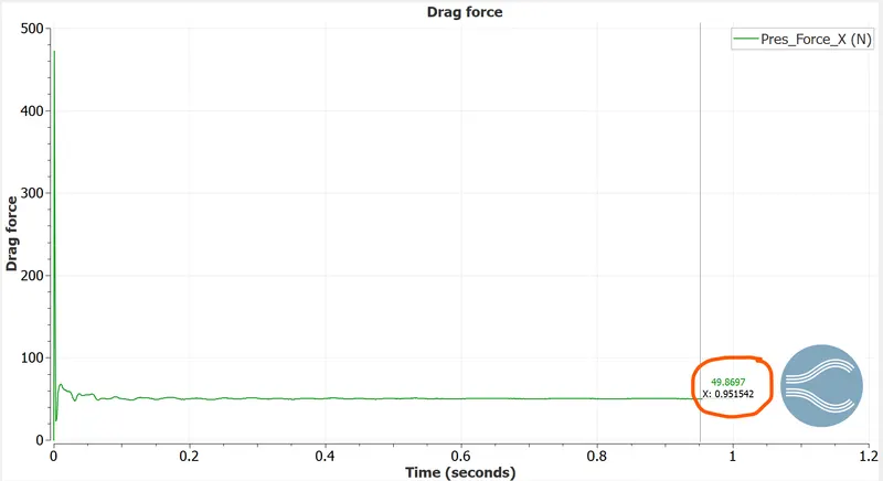
The drag force is 49.19 N
Correlation with converge plots
Lift force
Drag force
The coefficients of lift and drag can be calculated using the relation
`Funderset{d}{} = 1/2 * rho *Cunderset{d}{}* A*V^2 and Funderset{L}{} = 1/2 * rho *Cunderset{l}{}* A*V^2`
A = frontal area = 0.288 * 0.389 = 0.112 m^2.
rho = 1.225 kg/m^3
Cd = (2 * 49.19)/(1.225*40*40*.112) = 0.448
Cl = (2 * -241.12)/(1.225*40*40*.112) = -2.195
Conclusion
Thus the flow over the Ahmed body has been simulated, and the simulated data and the experimental data have been compared, and the coefficients of lift and drag have been calculated
The excel sheet and the setup file can be found under the link
https://drive.google.com/drive/folders/1ZwtKgVmHXy7ezWjsV-DHq9C8zQT0UohT?usp=sharing