Week 8 - Simulation of a backward facing step in OpenFOAM
Aim
To perform the simulation of backward facing step using OpenFOAM and compare the results of two different mesh growth factors - 1 and 0.2.
Theory
Geometry of backward facing step
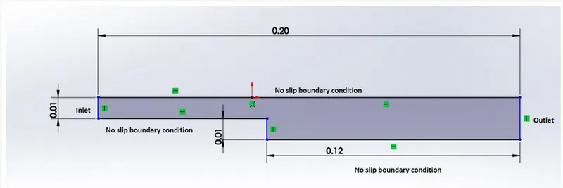
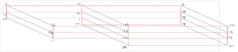
The above geometry has to be discretized into a number of blocks and combined together. The domain is divided into 5 blocks, as shown below
2D

3D
Solution
The simulation is found in the tutorials/incompressible folder in openFOAM. The name of the solver is icoFoam.
The relevant files are copied into a new folder under $FOAM_RUN. (eg:$FOAM_RUN/BFS_test1).
The folder cavity contains the relevant files for the simulation. The system folder contains the files "blockMeshdict" , "controlDict", "fvSchemes" and "fvSolution".
1. Blockmesh
The first step is to define the geometry using the coordinates of the vertices in the blockMeshdict file (using the gedit command). The vertices of all the faces are defined according to the right hand co-ordinate system, as shown below.
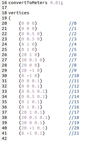
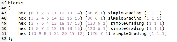
The blocks are created with 8 vertices, according to the right-hand coordinate system. The number of grid points in the X-direction are 80 for blocks 1 and 2, and 120 for 3,4 and 5, since the total number is 200. The number of grid points in the Y direction is 20 in the longer side, divided between the blocks. The grading factor is set to 1 in the simpleGrading values.
The inlets, outlets and walls are defined, as shown below.
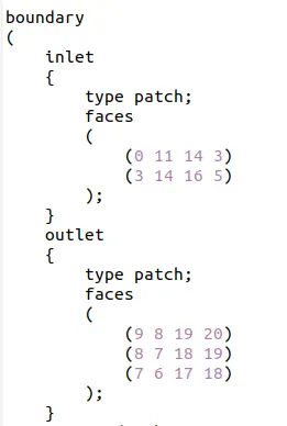
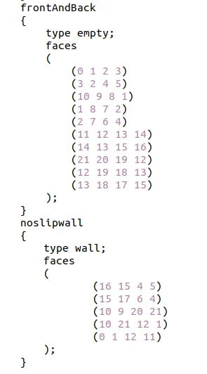
2. ControlDict
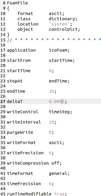
The timesteps and the runtime are given here, as shown below.
3. Velocity and Pressure
The velocity and pressure files are found in the 0 folder.
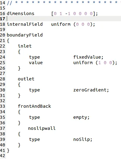
The initial velocity is 1 m/s. The velocity file is modified, as shown below.
Pressure
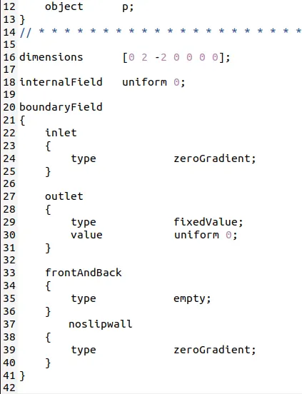
The mesh is now created using the blockMesh command, and the simulation is run using icoFoam.
The model can be opened in Paraview for post processing, using the paraFoam command.
Model with mesh

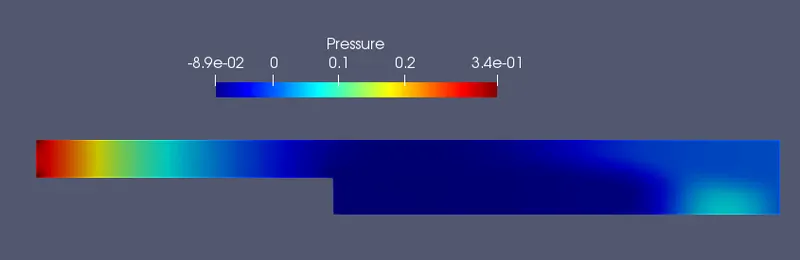
Pressure Contour
The pressure contour shows the high pressure initially and presence of low pressure in the middle part, due to fluid expansion. At the end of the flow, the pressure is again slightly higher.
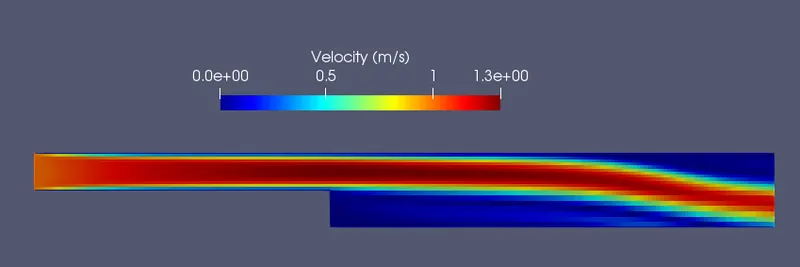
Velocity Contour
It can be seen, that the velocity is highest, in the middle region of the flow. Immediately after the step, the area is increased below the step, which leads to the formation of a recirculation region. The velocity here is zero, and decreases slightly from the maximum value near the neck.
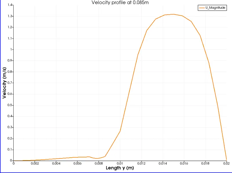
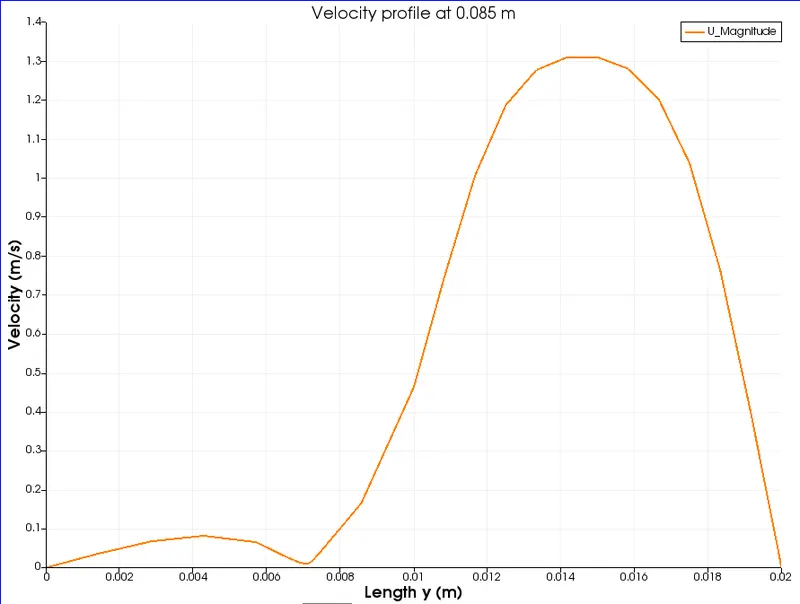
The value of the velocity at 0.085m can be found using the plot over line tool, as shown below.
The plot shows that the velocity profile is maximum at the middle part of the pipe and is close to zero, at the start and end of the pipe.
Grading factor 0.2
The blockmesh file is changed to get a finer mesh near the walls of the step. The script is shown below.
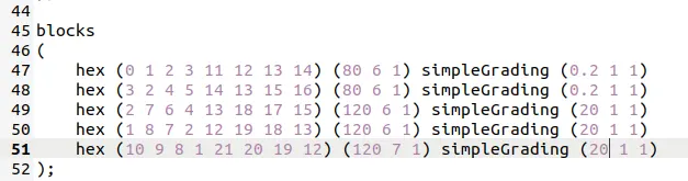
The rest of the parameters are the same. The model is simulated using the icoFoam command.
The model is viewed in Paraview for post processing.
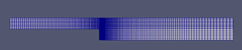
Model with mesh
The mesh can be seen with fine grading towards the walls of the step.
Pressure contour
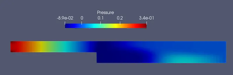
The pressure contour shows the high pressure initially and presence of low pressure in the middle part, due to fluid expansion. At the end of the flow, the pressure is again slightly higher.
Velocity contour
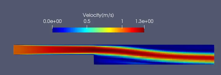
It can be seen, that the velocity is highest, in the middle region of the flow. Immediately after the step, the area is increased below the step, which leads to the formation of a recirculation region. The velocity here is zero, and decreases slightly from the maximum value near the neck.
The value of the velocity at 0.085m can be found using the plot over line tool, as shown below.
The plot shows that the velocity profile is maximum at the middle part of the pipe and is close to zero, at the start and end of the pipe.
Comparison between GF-1 and GF-0.2
On observation of the velocity profiles from both meshes, with grading factors 1 and 0.2, it can be seen, that the velocity profiles are very similar and no perceivable difference is present between the two.
Conclusion
The simulation of backward facing step of two different mesh growth factors - 1 and 0.2 is done, and the results are analyzed.