Week - 2 - Explicit and Implicit Analysis
Introduction:
Explicit and Implicit methods are numerical methods to solve a time-dependent differential equation.
Explicit method:
The value of the calculated variable at the previous time-step is used to calculate the required value at the current time-step. Explicit methods are conditionally stable, which means that the time-step selected has to be small in-order to satisfy the stability criterion (eg: Courant's condition, which states that the time-step must be smaller than an elastic wave to propogate from one side of the element to another.
Instead of verifying the global equilibrium, solver assumes that the equilibrium simply exists.This means that the solver goes straight into calculation of local finite element variables.It calculates all of the local finite element variables for given increment,and moves to the next one.
Example: In a force-displacement problem given by F = K.u, the displacement can be calculated by `u = (triangleF)/(triangleK)`, where F is the force matrix and K is the stiffness matrix. The value of the force at the previous time-step is used to approximate the displacement at the current time step given by
`u(n+1) = u(n) + trianglet.F(u(n))`
Explicit methods do not involve much computing cost, but the degree of accuracy is lesser compared to implicit methods.
Implicit method:
The value of the calculated variable at the current time-step is used to calculate the required value at the current time-step. Implicit methods are unconditionally stable, which means that there is no limitation on the size of the time-step.
Example: In a force-displacement problem given by F = K.u, the displacement can be calculated by `u = (triangleF)/(triangleK)`, where F is the force matrix and K is the stiffness matrix. The value of the force at the current time-step is used to approximate the displacement at the current time step given by
`u(n+1) = u(n) + trianglet.F(u(n+1))`
`(I-A)triangleT.u(n+1) = u(n)`
On the other hand, the implicit methods involve higher cost of computation, since matrix inversion is involved at each step, but with a higher degree of accuracy compared to explicit methods.
Given Problem:
`F(u) = u^3 + 9u^2 + 4u`
Therefore,
`K(u) = 3u^2 + 18 u + 4`
The above problem has been solved by both explicit and implicit methods as follows:
Explicit method:
Here,three equal load increments (or steps) of ∆F = 1 unit each are used to load the tension bar.
The variables used are u for displacement, f for internal force in the bar, F for external force applied to the bar and k for stiffness. Incremental displacements or incremental externally applied forces are represented as ∆u or ∆F, respectively. Use is made of
the relationship ∆F=k∆u. The analysis proceeds as follows:
Step − 1
`u0 = 0.0, k(u0) = , triangle F = 1, triangle u = (triangle F)/(k(u0)) = 0.25, u1 = u0 + triangle u1 = 0.25`
`F external = triangle F = 1`
`F Internal = u^3 + 9u^2 + 4 u = 1.5781 (because u = u1)`
Step − 2
`u1 = 0.25, k(u1) = 8.675, triangle F = 1, triangle u = (triangle F)/(k(u1)) = 0.1151, u2 = u1 + triangle u2 = 0.3611`
`F external = triangle F + triangle F = 2`
`F Internal = u^3 + 9u^2 + 4 u = 2.7088 (because u = u2)`
Step − 3
`u2 = 0.3651, k(u2) = 10.9718, triangle F = 1, triangle u = (triangle F)/(k(u2)) = 0.0911, u3 = u2 + triangle u3 = 0.4562`
`F external = triangle F + triangle F + triangle F = 3`
`F Internal = u^3 + 9u^2 + 4 u = 3.7934 (because u = u3)`
It is evident from the results that external and internal forces are NOT in equilibrium because F external `F external ne F Internal` .
The following table summarizes the results for explicit analysis method.
| Step | ∆F | ∆u | u | Fext | Fint | R = Fint- Fext |
| 1 | 1 | 0.25 | 0.25 | 1 | 1.578125 | 0.578125 |
| 2 | 1 | 0.115108 | 0.365108 | 2 | 2.708836 | 0.70883602 |
| 3 | 1 | 0.091142 | 0.45625 | 3 | 3.793454 | 0.793454169 |
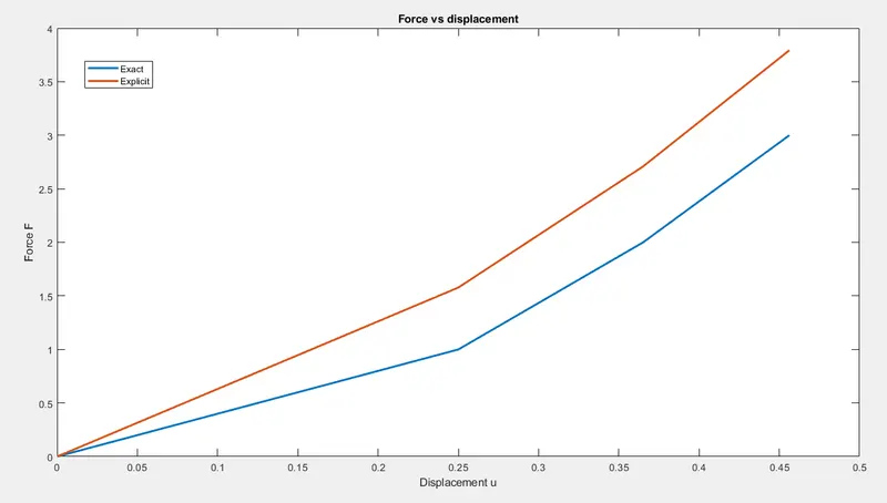
From the plot it can be very clearly seen, that the explicit solution does not converge with the exact solution.
Implicit method:
An implicit analysis is the same as the explicit analysis, except that at the end of each step Newton-Raphson iterations are usedto enforce equilibrium before moving to the next step.
Basically, an incremental force is applied to advance the solution forward at the beginning of a step. However, internal forcesand external forces will not be in equilibrium unless the
stiffness is linear for the given step.
Hence, in order to achieve equilibrium, corrections must be made to the displacement.
This is accomplished by using Newton-Raphson iterations to minimize the residual `R = F Internal - F external`,
Expanding the residual as a Taylor series about the current displacement `u^j` gives
`R^(j+1) = R^j (u^j) + (dR(u^j))/(du).deltau^(j+1) + ..... = R^j + k(u^j).deltau^(j+1) + ....`
By neglecting higher order terms in the series, setting `R^(j+1) = 0` and solving for `deltau^(j+1)`the following correction is obtained.
`deltau^(j+1) = - [k(u^j)]^-1.R^j`
Here, the iteration variable is j and it may take several iterations for the norm of the residual, R, to be reduced below the chosen
tolerance criteria of 0.01.
The implicit analysis proceeds as follows
Step - 1
`u0 = 0.0, k(u0) = 4, triangle F = 1, triangle u1 = (triangle F)/k(u0) = 0.25, u1 = u0 + triangle u1 = 0.25`
`F external = triangle F = 1`
`F Internal = u1^3 + 9 u1^2 + 4 u1 = 1.578125`
Checking the residual
Residual `R1^((0)) = F Internal - F external = 0.578125`
`R1^((0)) > 10^-2 implies`Newton Raphson iterations are necessary.
Calculation of correction `u1 = u1^((0))`
`delta u^((1)) = - [k(u1^((0)))]^-1.R1^((0)) = -(8.6875)^-1 .0.578125 = -0.06654``implies u1^((1)) = u1^((0)) + deltau^((1)) = 0.25 - 0.06554 = 0.1834`
Checking the residual again,
`F external = triangle F = 1`
`F Internal = (u1^((1)))^3 + 9( u1^((1)))^2 + 4 u1^((1)) = 1.04288`
Residual `R1^((1)) = F Internal - F external = 0.04288`
`R1^((1)) > 10^-2 implies`Newton Raphson iterations are necessary.
Calculation of correction `u1 = u1^((0))`
`delta u^((2)) = delta u^((1))- [k(u1^((1)))]^-1.R1^((1)) = -0.06654 - (7.4031)^-1 .0.04288 = -0.0723``implies u1^((2)) = u1^((0)) + deltau^((2)) = 0.25 - 0.0723 = 0.1776`
Checking the residual again,
`F external = triangle F = 1`
`F Internal = (u1^((2)))^3 + 9( u1^((2)))^2 + 4 u1^((2)) = 1.0003`
Residual `R1^((2)) = F Internal - F external = 0.0003`
`R1^((2)) < 10^-2 implies`Newton Raphson iterations are not necessary.
The final value of `u1 = u1^((2)) = 0.1776`
Step - 2:
`u1 = 0.1776, k(u1) = 7.2925, triangle F = 2, triangle u2 = (triangle F)/(k(u1)) = 0.1371, u2 = u1 + triangle u2 = 0.3147`
`F external = triangle F + triangle F = 2`
`F Internal = u2^3 + 9 u2^2 + 4 u2 = 2.1821`
Checking the residual
Residual `R2^((0)) = F Internal - F external = 0.1822`
`R2^((0)) > 10^-2 implies`Newton Raphson iterations are necessary.
Calculation of correction `u1 = u1^((0))`
`delta u^((1)) = - [k(u2^((0)))]^-1.R2^((0)) = -(9.9634)^-1 .0.1821 = -0.01828``implies u2^((1)) = u2^((0)) + deltau^((1)) = 0.3147 - 0.01828 = 0.2965`
Checking the residual again,
`F external = triangle F + triangle F = 2`
`F Internal = (u2^((1)))^3 + 9( u2^((1)))^2 + 4 u2^((1)) = 2.003`
Residual `R2^((1)) = F Internal - F external = 0.0033`
`R2^((1)) < 10^-2 implies`Newton Raphson iterations are not necessary.
The final value of `u2 = u2^((1)) = 0.2965`
Step 3:
`u1 = 0.2965, k(u1) = 9.6008, triangle F = 1, triangle u3 = (triangle F)/(k(u2)) = 0.1041, u3 = u2 + triangle u3 = 0.4006`
`F external = triangle F + triangle F + triangle F = 3`
`F Internal = u3^3 + 9 u3^2 + 4 u3 = 3.1117`
Checking the residual
Residual `R3^((0)) = F Internal - F external = 0.1117`
`R3^((0)) > 10^-2 implies`Newton Raphson iterations are necessary.
Calculation of correction `u1 = u1^((0))`
`delta u^((1)) = - [k(u3^((0)))]^-1.R3^((0)) = -(11.6942)^-1 .0.1117 = -0.00956``implies u3^((1)) = u3^((0)) + deltau^((1)) = 0.4006 - 0.00956 = 0.3911`
Checking the residual again,
`F external = triangle F + triangle F + triangle F = 3`
`F Internal = (u3^((1)))^3 + 9( u3^((1)))^2 + 4 u3^((1)) = 3.0009`
Residual `R3^((1)) = F Internal - F external = 0.00093`
`R3^((1)) < 10^-2 implies`Newton Raphson iterations are not necessary.
The final value of `u3 = u3^((1)) = 0.3911`
The results of the implicit analysis are summarized in the table below
| Step | ∆F | u | Fext | Fint | R = Fint- Fext |
| 1 | 1 | 0.1776607 | 1 | 1.000320254 | 0.00032 |
| 2 | 1 | 0.29650431 | 2 | 2.003317615 | 0.003318 |
| 3 | 1 | 0.39110656 | 3 | 3.000930646 | 0.000931 |
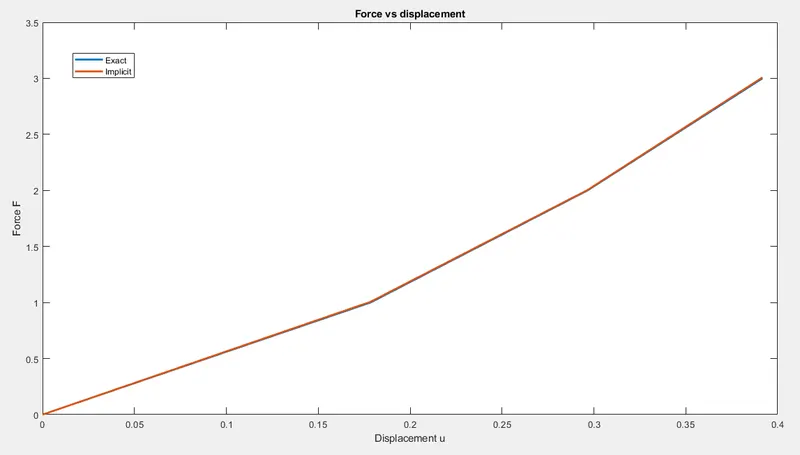
From the above plot, it can be very clearly seen that the implicit solution converges with the exact solution.
The excel sheet with the calculations and the plots can be found under the link below
https://drive.google.com/drive/folders/19ScDmR4ylO_L-Z613uIirWGNCVI-Fp8h?usp=sharing