Crash Box Simulation

Objective:

To set up solver input and output requests for the Crash box with different thicknesses as1.2mm and 1.5mm and study the behavior of the crash box when crushing on a Rigid wall. Then we need to get the results as follows.

-Input .k file and output files (d3plot, glstat, sleout, rcforc)

- Animation of the final simulation

- Cross-sectional force generated in the middle of the crash box (along its length)

- Acceleration plot of a node in the middle of the crash box (along its length)

- Maximum directional stress and strain along the length of the crash box (X strain, Y strain, etc)

- Plot of all energies (total, internal, kinetic, hourglass, sliding)

- Compare the accelerations and stress/strain plots of 1.2/1.5mm crash boxes.

Procedure:

Case setup:

Here we have .K keyword file with only mesh with basic node, element, part keywords only. So we need Set up the solver keywords for the model and give end time for the solver and Give output requests for the graph and animation files.

At first, import the keyword file using File>open>Ls_dyna keyword file in LS-Prepost.

Creating Material card:

Case:1_Crash box_1.2mm:

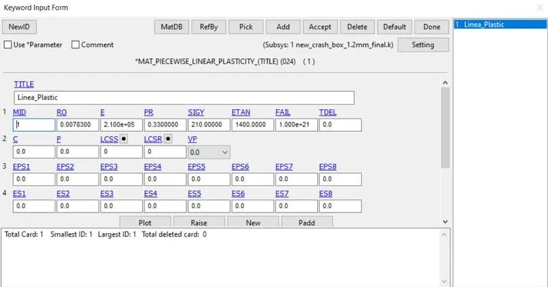
To create material cards for the crash box. By clicking Model & part>keywords>all>MAT>Mat-24 piecewise >assign values of (material id, RO, Young’s modulus, Poisson’s ratio, ETan, SigY)>accept>done. Here we assigned steel material values for the material card. The same material card was also used for case-2.

Creating section card:

Case:1_Crash box_1.2mm:

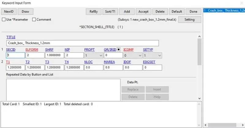
First, we need to assign a Section id for the model. By clicking Model & part>keywords>all>section>shell. Now assign values and click accept and done. Assign thickness as 1.2mm.

Case:2_Crash box_1.5mm:

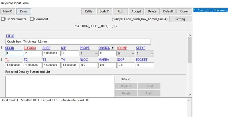
Here same values were assigned for the material except for thickness as 1.5mm.

Assigning section id and MAT id for case 1 and case 2:

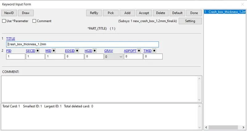
Now assign material and section cards for the parts using Model & part>keywords>Part>assign SECID, MID>accept>done.

Creating contact card for case-1 & case-2:

Here we have the same contact card for both cases. At first, we need to create a node-set for assigning the control card.

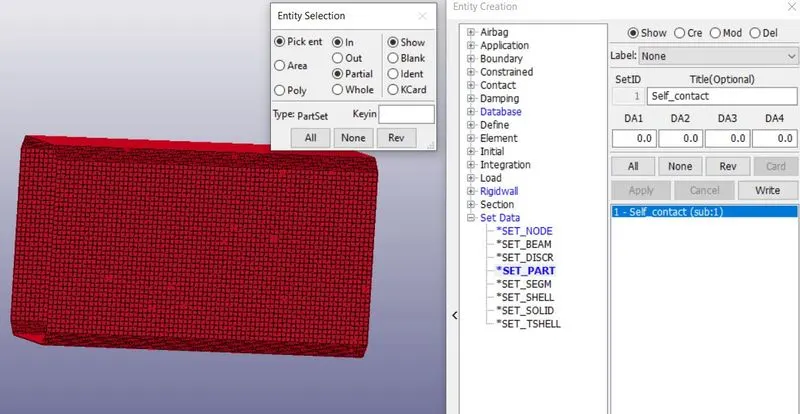
For part set id creation, go to Model & part>Create entity>Set data>set part>create>pick by part>assign a title and set id>apply>done.

We need to assign a set id and title and then pick the parts using the part tool. After that click apply and done.

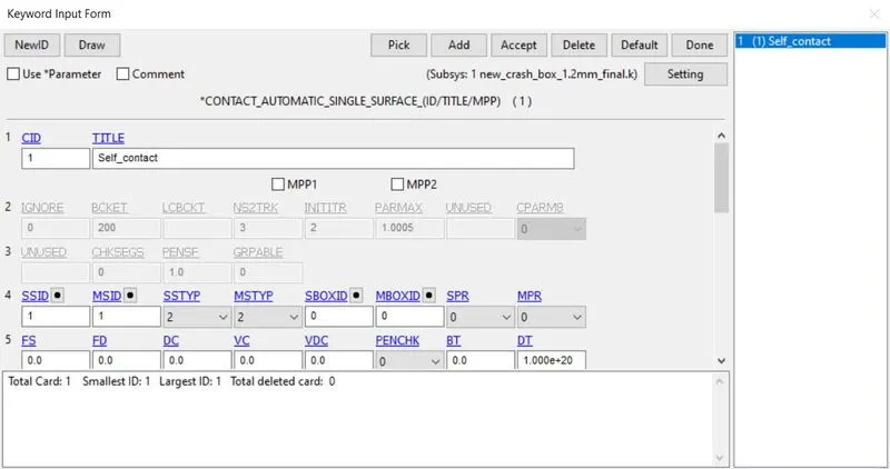
Here we need to assign self contact for the model. So we can give only slave set id to assign self contact by clicking Model & part>keywords>Contact>Automatic_single_surface. Assign the slave set id type as 2 for part set id and put SSID value. Click accept and done.

Creation of Rigidwall:

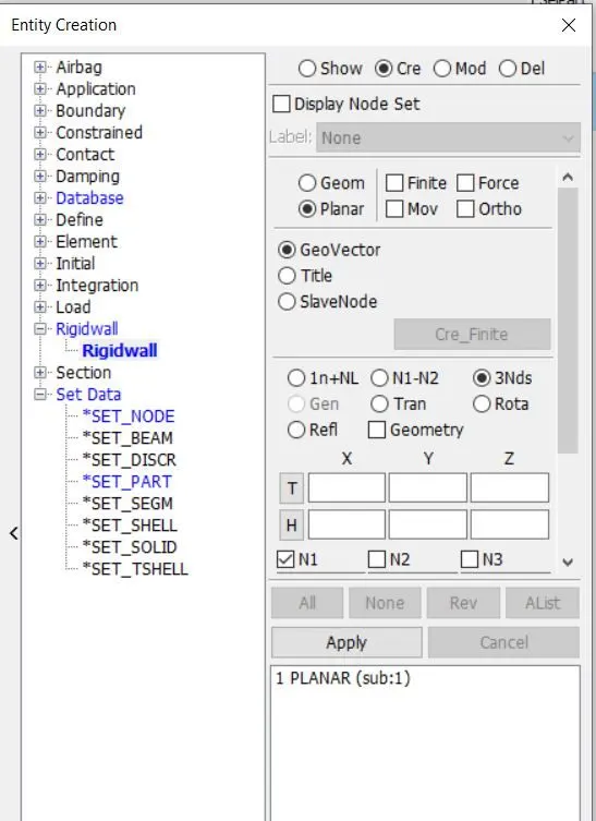
Here we need to crash the box using rigid wall. So we need to create a rigid wall using Model & part>Create entity> Rigid wall. Now select planar and select 1n+nl. After that Click one node at one end and assign -10mm at x-axis translational from that node. now apply and done.

Assigning initial velocity for the crash box:

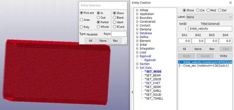
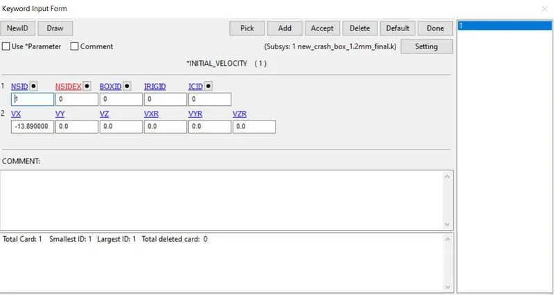
At first, we need to create a node-set for assigning initial velocity. For Node set id creation, go to Model & part>Create entity>Set data>set node>create>pick by part>assign a title and set id>apply>done. We need to assign a set id and title and then pick the nodes using the part tool. After that click apply and done.

Now go to Model & part>keywords>initial>velocity. Assign value as -13.88mm/ms (50kmph) through x-axis and assign node-set id value. Now accept and done.

Creating Cross-section for both cases:

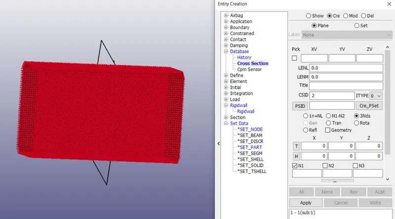
Now go to Model & part>Create entity>database>cross-section. Now select create>plane>3nds. Now click three nodes to assign a plane parallel to the rigid wall. Click apply and done. Now the cross-section was created.

Creating History node for particular node:

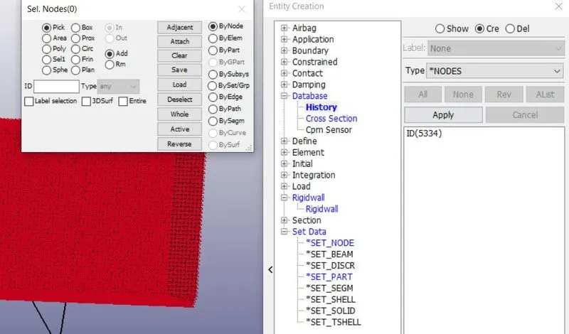
Now go to Model & part>Create entity>database>History >create>node. Now pick the node and select apply and done. Now a node was assigned.

Creating output requests:

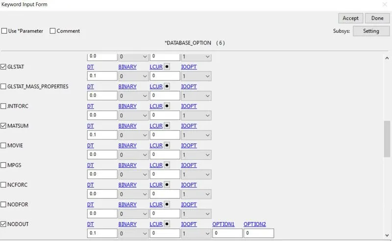
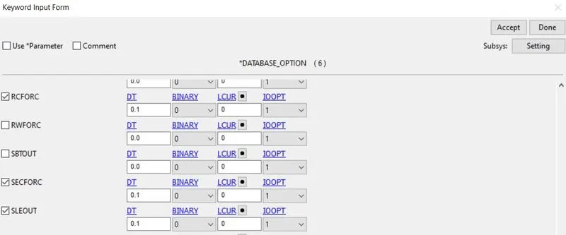
Now we need to give output requests for the graphs we want to plot. By clicking Model & part>keywords>Database>ASCII. Here we need to assign DT for GLSTAT, MATSUM, RCFORC, NODOUT, SECFORC, SLEOUT. Assign DT value as 0.1ms.

Creating animation output file:

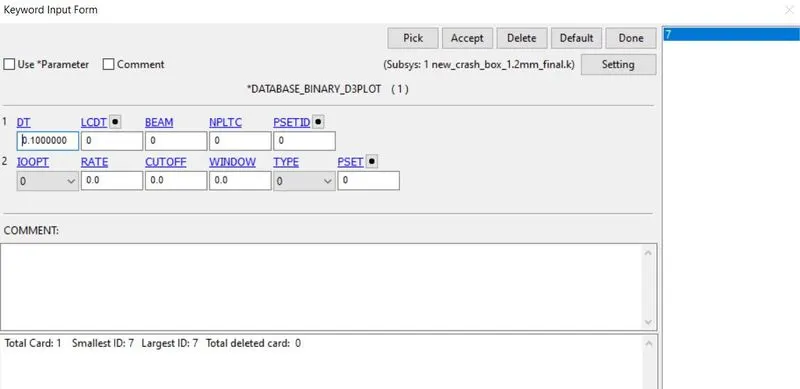
we need to give output requests for the aimation. By selecting Model & part>keywords>Database>Binary D3plot. Here assign DT value as 0.1ms.

Creating control termination card:

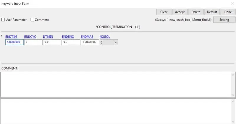
We need to put end time for the simulation for that select Model & part>keywords>Control>termination. Now assign end time as 5ms.

Post-processing results:

D3plot:

Here we need to show the animation of the model. So go to Open>ls-dyna binary plot. Now select post>fringe component>Von-mises stress. now select dynamic in Fringe range. The animation shows below

Case:1_1.2mm:

Von mises stress animation:

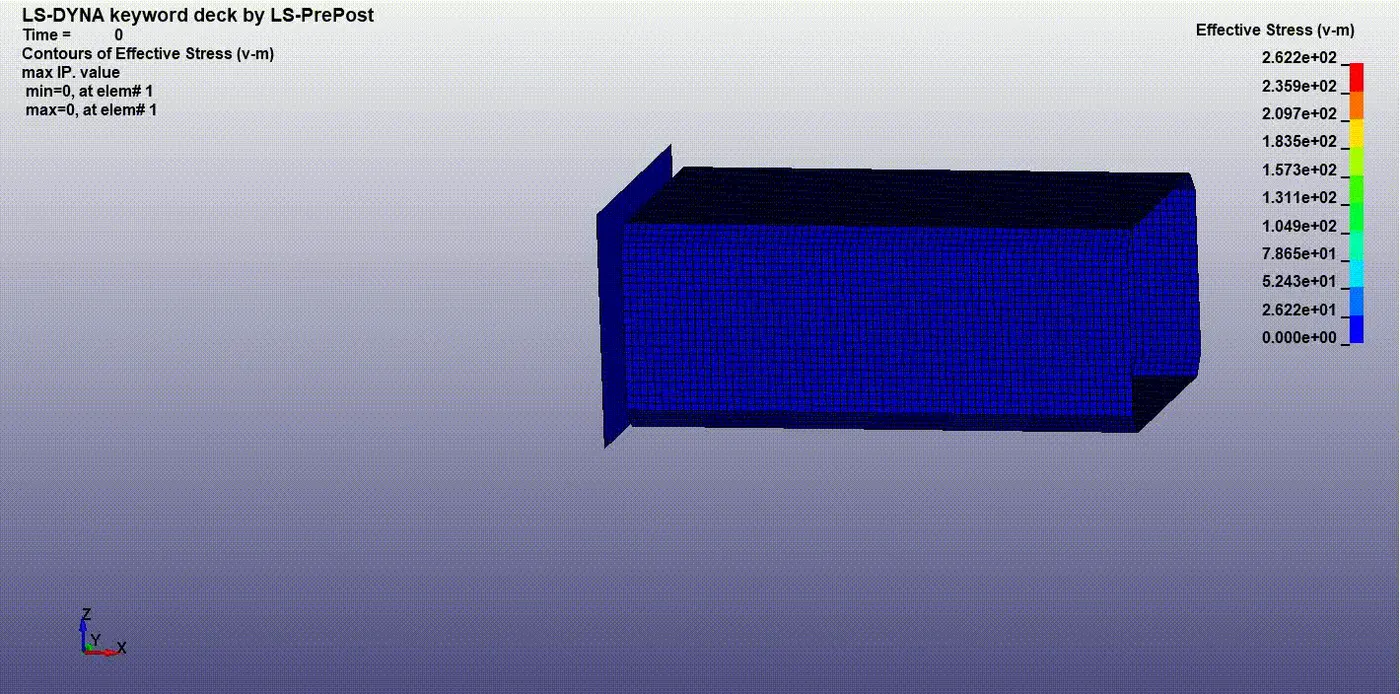
The animation shows that the maximum stress occurs at 0.2622pa. During the impact, the crash box was impacted on the rigidwall at the velocity of 13.88mm/ms. At initial, the elements got maximum stress during the imapct time. The stress were transferred to the other elements during the rebound.

Effective plastic strain:

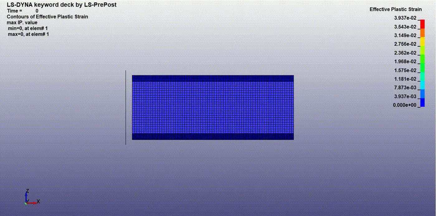
The Plastic strain value was maximize at 0.039mm which was lesser value. so that strain rate was lower due to the rebound activity. if the crash box impact the rigidwall and crushed on it. the strain will be high due to the large deformation.

Case-2_1.5mm:

Von mises stress animation:

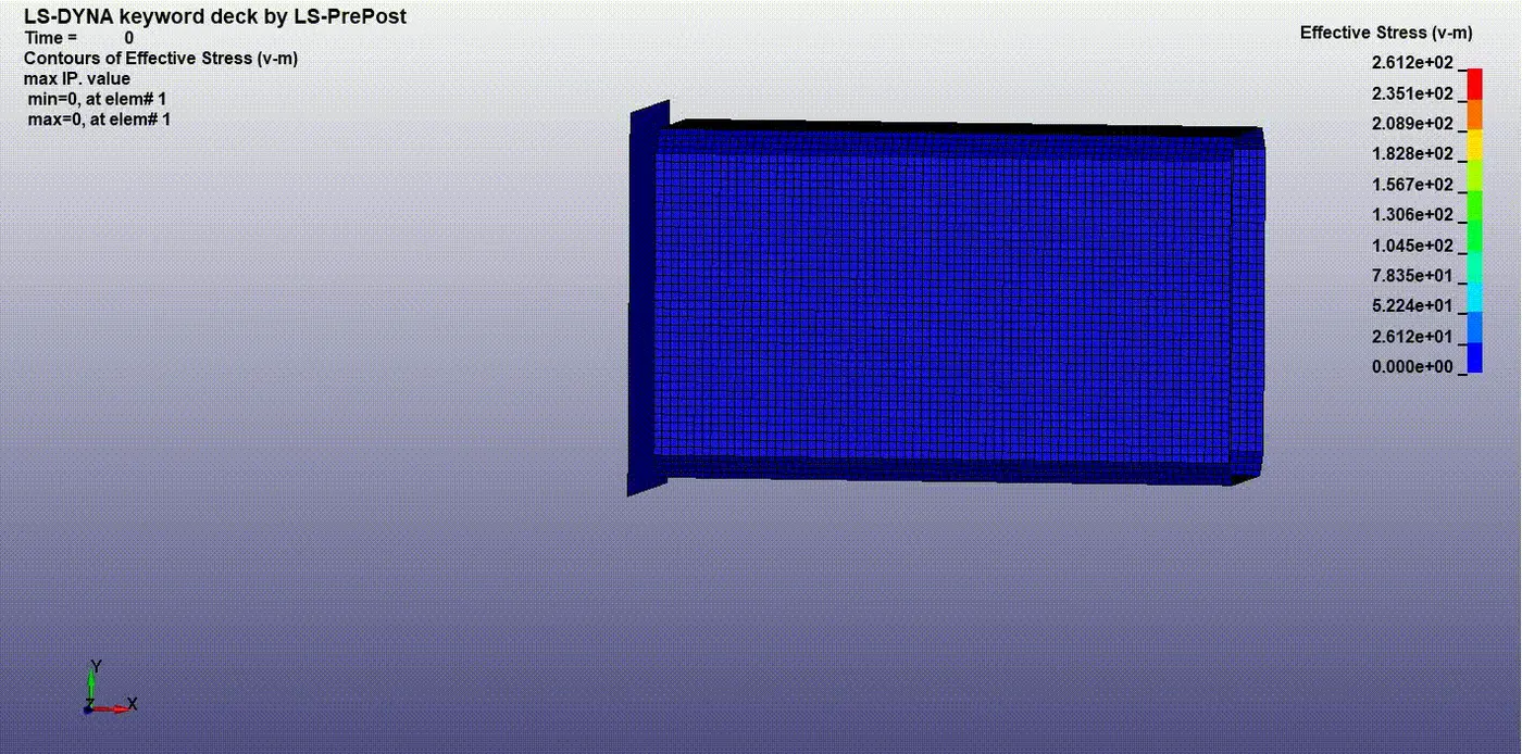
The animation shows that the maximum stress occurs at 0.2612pa. Here we have slight variation in the stress value due to the thickness of 1.5mm. so that the thickness increases, the stress induced in the system decreases.

Effective plastic strain:

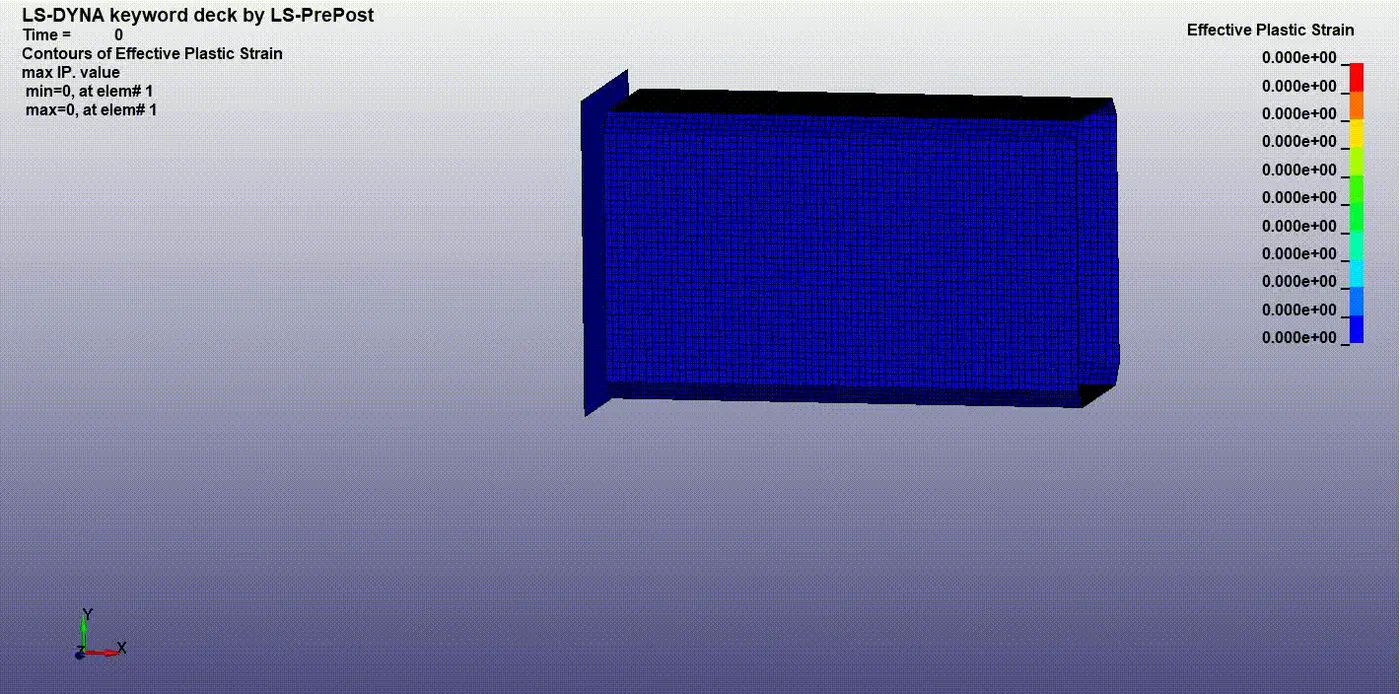
The plastic strain value is 0.0386mm. the strain rate also got slight variations due to thickening the part.

Comparison of acceleration of the node:

Case:1

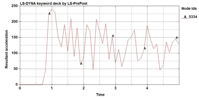
Here the acceleration wad induced on node 5334 at 245mm/ms^2 in 1ms because at that time, the crash box got impacted in the wall due to the impact, the node accelerated at high rate.

Case:2

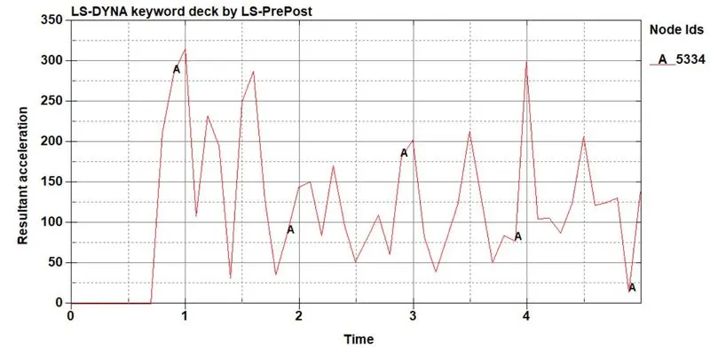
Here the acceleration wad induced on node 5334 at 320mm/ms^2 in 1ms. The acceleration had higher vlaue than case-1. Due to the thickness of model, the acceleration of the node 5334 was increased drastically.

Comparison of cross section force of both cases:

Case:1

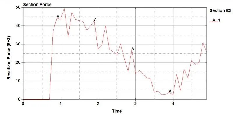
The resultant force of the cross section at 49 gm*mm/ms^2. At the time of impact, the cross section got the maximum force at 1.1ms.

Case:2

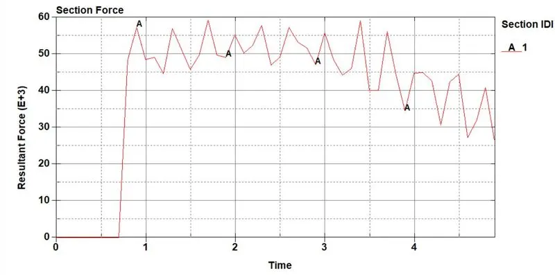
The resultant force of the cross section at 59 gm*mm/ms^2. At the time of impact, the cross section got the maximum force at 1.7ms. Due to the high thickness, the model got delayed to get a maximum force at the time of imapct.

Comparison energy graphs of both cases:

Case:1

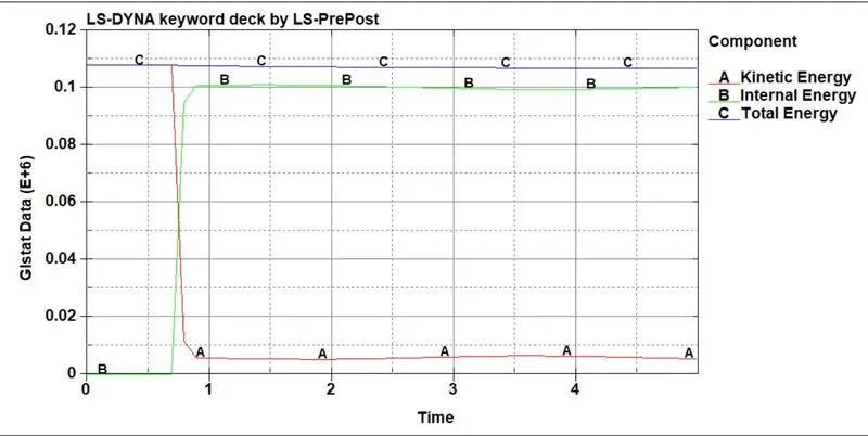
Here we have energy graphs, the maximum internal energy is at 0.1J of 0.9ms. the kinetic energy was maximize at starting at 0.11J.at that time, the kinetic energy was decreased due to absorbtion of energy when the model got impacted into the wall. the kinetic energy were transferred to internal energy of the model. the total energy got constant due to the balance in both the energies.

Case:2

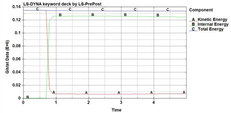
The maximum kinetic energy is at 0.13J of starting time. the internal energy was maximize at 0.9ms at 0.125J.at that time, the kinetic energy was decreased due to absorbtion of energy when the model got impacted into the wall.Due to the variations of thickness, the energy had higher values than case 1. the total energy got constant due to the balance in both the energies.

Conclusion:

The given crash box was analyzed using different type of thickness at 1.2mm and 1.5mm. The energy graphs shows that higher energy induced in larger thickness during the impact. so that the thickness plays a major role in the analysis of the crash box. The acceleration and section force are compared in the results. the stress and strain values are compared in the above results.