Calculate the Stretch Ratio by comparing the ELFORM (-2,-1,1,2) with Ogden_Material Model.

Objective:

• To Create a block of 10mmx10mmx10mm dimension with 10 elements for each direction and use the material card attached (Ogden_Material.k)
• To Use appropriate boundary conditions to simulate tensile behavior for the model.
• To compare the results for the simulation using ELFORM = 1, 2, -1, -2 and Use a proper solver (Implicit/Explicit).

Procedure:

Theory:

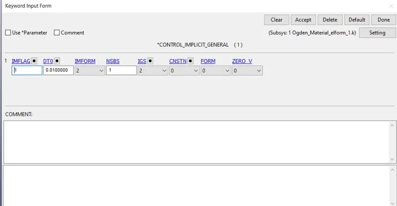
Here we used an implicit solver for simulation because the analysis is quite similar to the quasi-static analysis on Ogden material (hyper-elastic non-linear material) with slow loading conditions. We need to change the Iflag parameter as 1 for implicit analysis in the control_implicit_general keyword card.

Case setup:

Open LS-Dyna pre post, select file>open>LS-Dyna keyword file. Now select the given keyword file.

The keyword consists of only MAT card and TITLE card. So we need to create a solid box part using the given parameters.

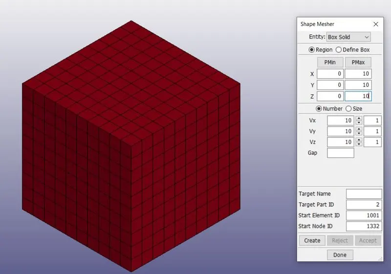
Now select Mesh>shape mesher. Now create a FE solid block of 10mm*10mm*10mm dimension of each direction has 10 elements.

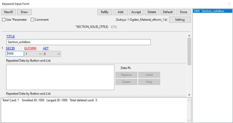
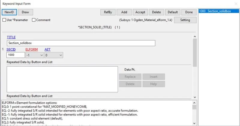
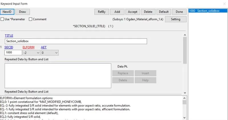
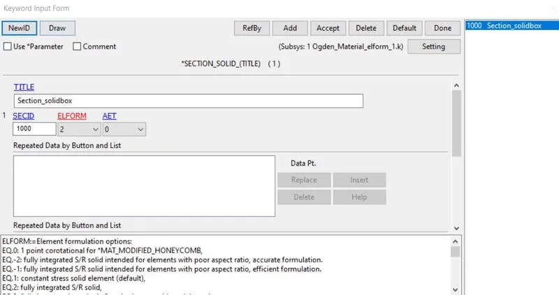
Now create section id for the part using Model & part>keywords>Section_solid. Now assign sec id and Elform as 1. After that, we need to change elform as 2, -1, -2 for the other three cases.

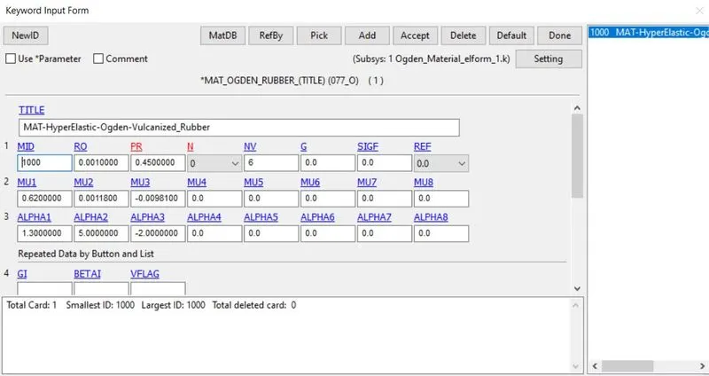
MAT id for the part is given below,

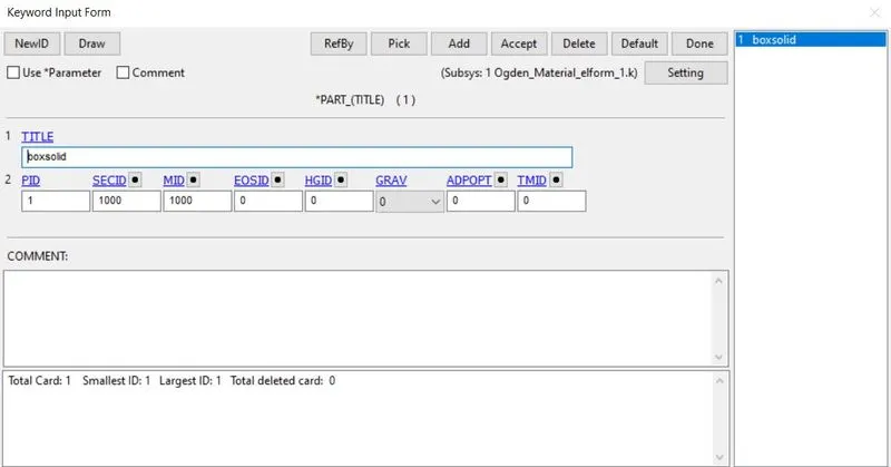
Now define both sec id and Mat id for the part using Model & part>keywords>part.

Defining boundary conditions:

To perform the tensile test on the part. We need to lock DOF’s of one face and define displacement for the other face.

For that, first, we need to define the node-set for the Boundary_spc to lock X-axis translational and all rotational axis. Now define all the nodes of the face using create entity>set data>set node>select the nodes>apply>done.

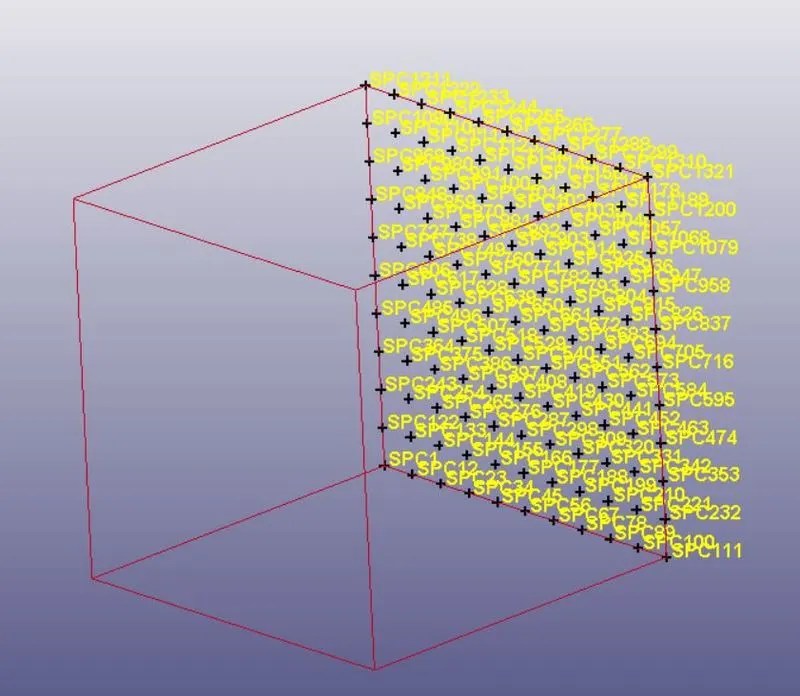
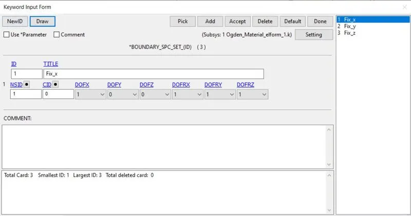
Now we should define boundary_spc for the node-set using Model & part>keywords>boundary_spc_set. Now define Node set id and translational x-axis type as 1 and lock all rotational DOF’s.

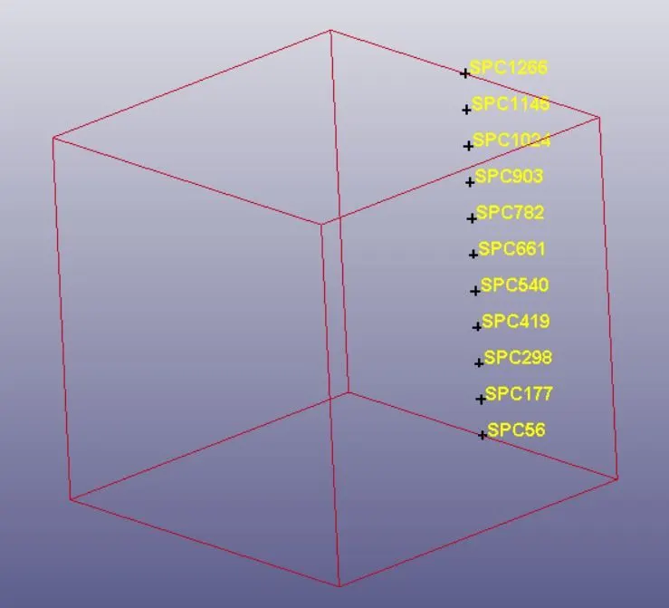
Now we need to define the node-set for the Boundary_spc to lock y-axis translational and all rotational axis. Now define one set of vertical nodes at the center of the face using create entity>set data>set node>select the nodes>apply>done.

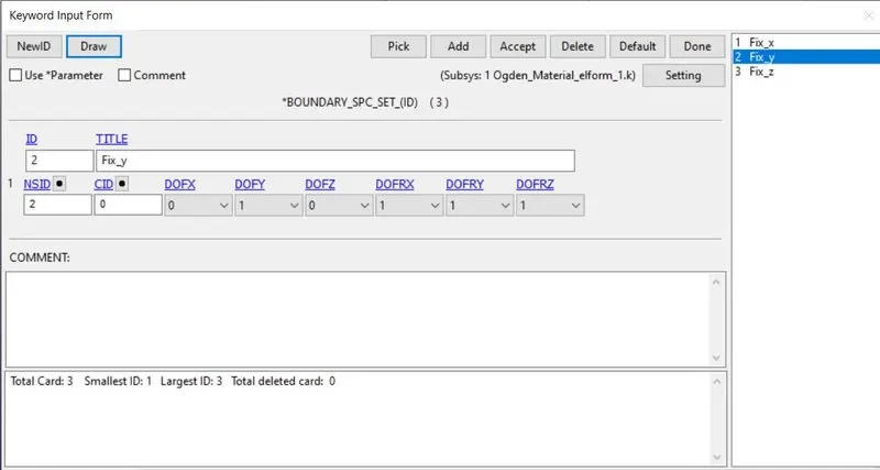
Now we should define boundary_spc for the node-set using Model & part>keywords>boundary_spc_set. Now define Node set id and translational y-axis type as 1 and lock all rotational DOF’s.

Now define one set of horizontal nodes at the center of the face using create entity>set data>set node>select the nodes>apply>done.

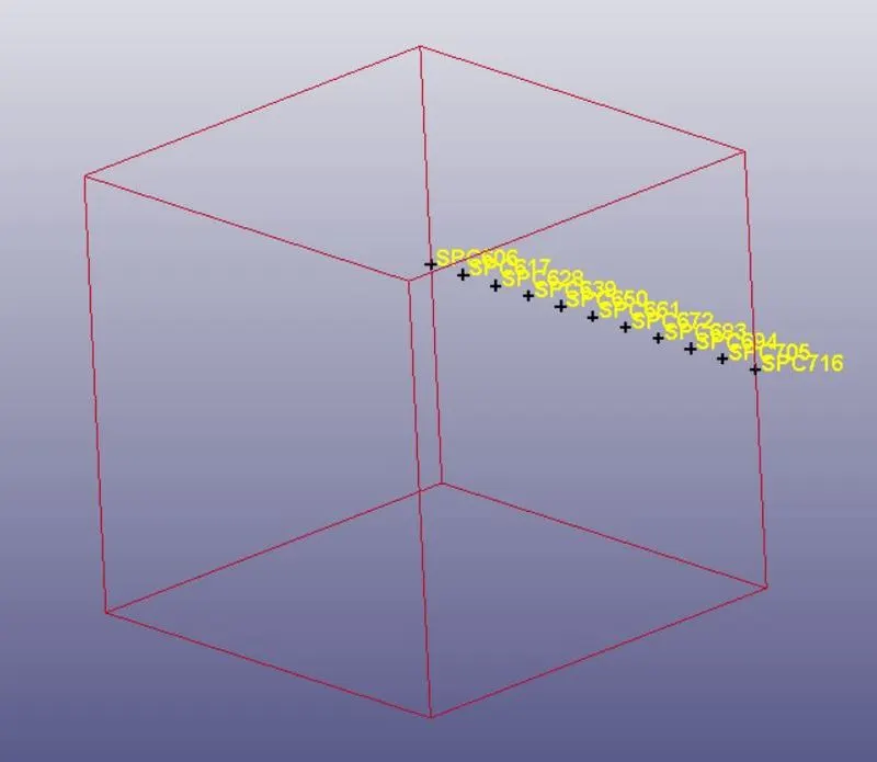
Now we should define boundary_spc for the node-set using Model & part>keywords>boundary_spc_set. Now define Node set id and translational z-axis type as 1 and lock all rotational DOF’s.

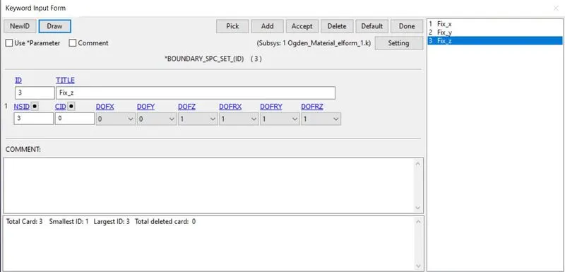
Before defining displacement we need to define a curve for the displacement. For that, Model & part>keywords>Define>curve. The plotted curve is shown below.

For displacement,

The stretch ratio is 5,

Engineering strain,`epsilon`e=`deltal/l`

Stretch ratio, `lamda=1+epsilone`

`5=1+deltal/10`

`deltal=40mm`

the displacement value is 40m.

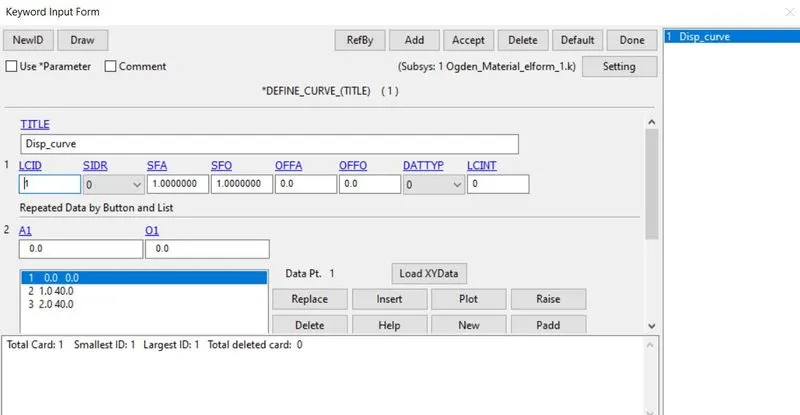
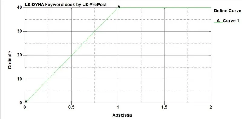
For Displacement, first, define all the nodes of the other face using create entity>set data>set node>select the nodes>apply>done.

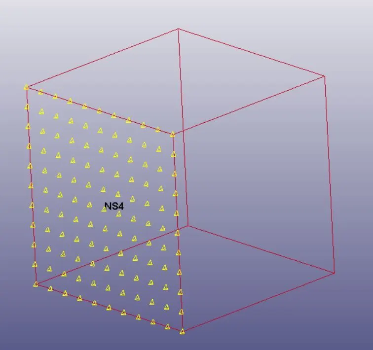
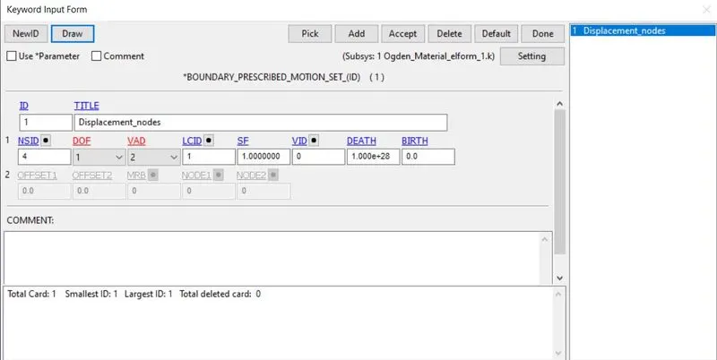
Now we should define boundary_prescribed_motion for the node-set using Model & part>keywords>boundary_prescribed_motion_set. Now define Node set id and translational x-axis type as 1 and VAD flag type as 2 for displacement and define curve id. Now select done.

Defining Database cards:

Go to Model & part>keywords>Database for defining the below cards.

For Binary D3plot, Assign the DT value as 0.01ms.

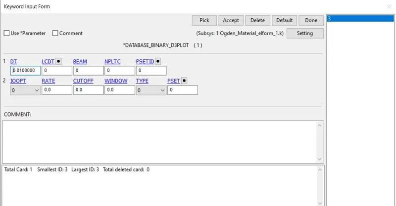
For ELOUT, GLSAT, NODOUT, Assign DT value as 0.01ms

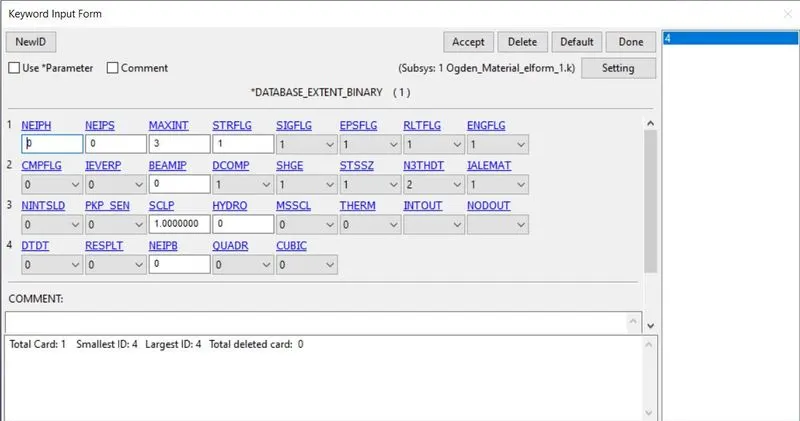
For DATABASE_BINARY_EXTENT, Assign STRFLG-1 and it is used to compute the strain values.

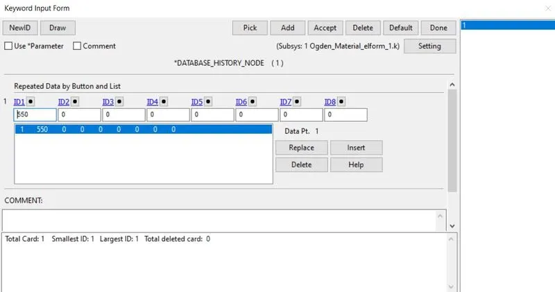
Now assign DATABASE_HISTORY_NODE using create entity>Database>history and select the node and apply done.

Defining control cards:

Go to Model & part>keywords>Control for defining the below cards.

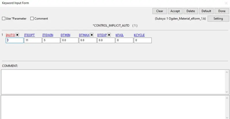
Control_implicit_auto is used to control time steps automatically during the implicit analysis. The input parameter of IAuto is 1.

Control_Implicit_general is used to activate the implicit analysis. Input parameters are IMFlag-1 and DTO-0.01ms.

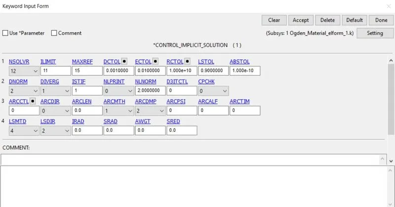
Control_implicit_solution is used to assign linear or non-linear solutions. Assign the default values.

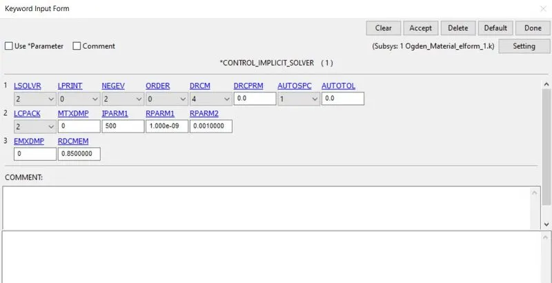
Control_implicit_solver: Assign the default values.

Control termination:

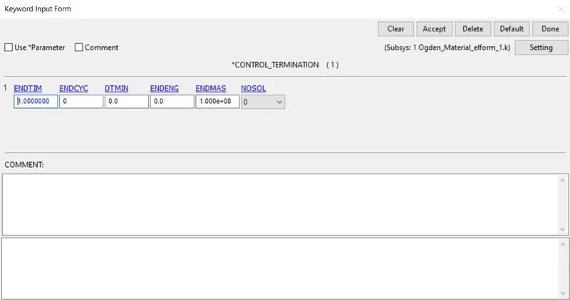
Here assign the end time of the simulation as 1ms.

Results:

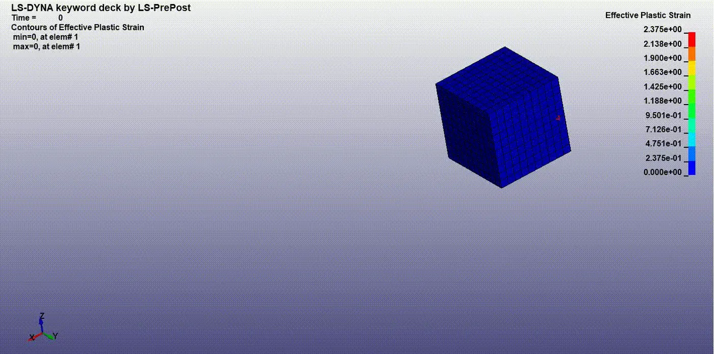
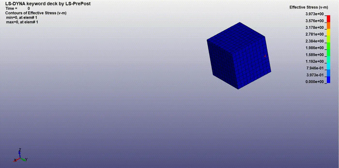
1. open LS-Pre post. NOw open>LS-Dyna binary plot. D3plot file in the same directory folder. After open the file, we need select Post>frige component>stress>von-mises stress @ effective plastic strain>Apply. Now the animation file is shown below.

Case_1 Elform_1:

Effective plastic strain:

Von mises stress:

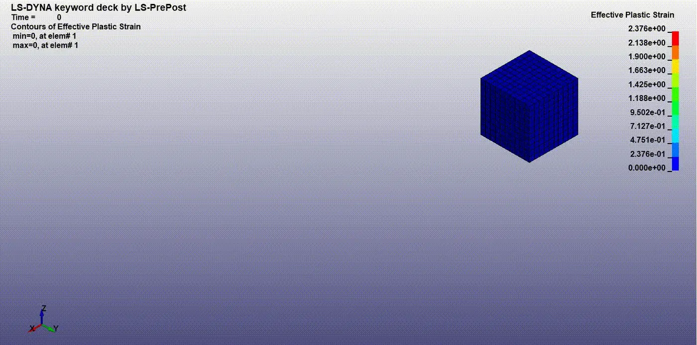
Case_2 Elform_-1:

Effective plastic strain:

Von mises stress:

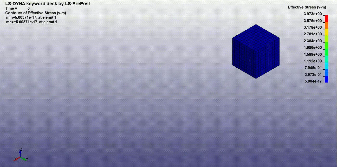
Case_3 Elform_-2:

Effective plastic strain:

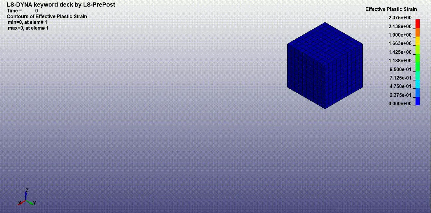
Von mises stress:

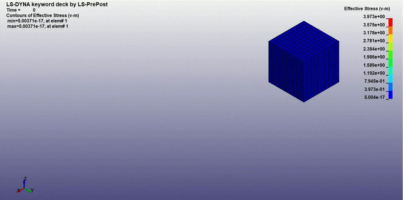
Case_4 Elform_2:

Effective plastic strain:

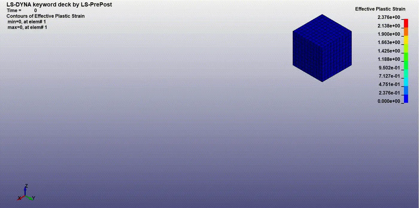
Von mises stress:

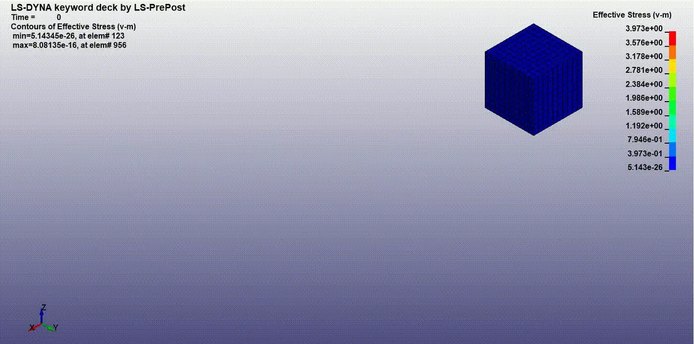
The maximum stresses induced in the above cases are 3.97Mpa around. it is pretty much similar to all the cases above. The effective plastic strain is also pretty much similar to all cases it's around 3.97mm. The maximum stresses in the above cases have slight variations in the stress level but the strain level is almost the same for different kinds of elforms.

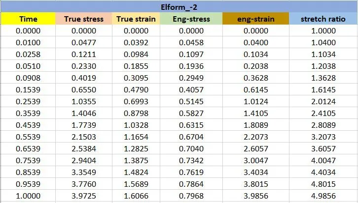
2. Calculating engineering stress & strain values and stretch ration for all cases:

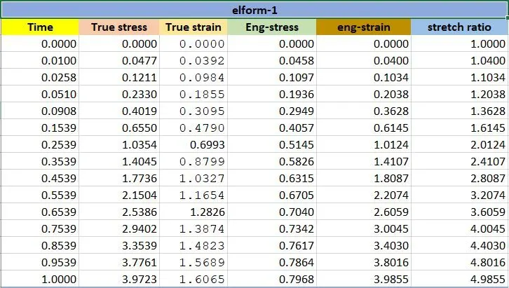
In LS-Dyna prepost, we can get stress & strain values using Post>fringe component that values are true stress & strain values. But to find Engineering stress and strain values & stretch ratio following relations are used,

We know true stress & strain values so using this we can get engineering stress & strain values.

True stress, `sigmat=sigmae(1+epsilone)`

True stain, `epsilont=ln(1+epsilone)`,

Similarly, Engg stress, `sigmae=sigmat/(1+epsilone)`

Engg strain, `epsilone=e^epsilont-1`

Stretch ration, `lamda=1+epsilone`

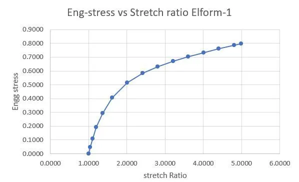
Engineering stress vs stretch ratio plot for Elform_1

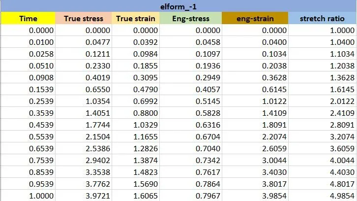
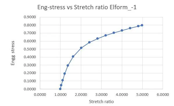
Engineering stress vs stretch ratio plot for Elform_-1

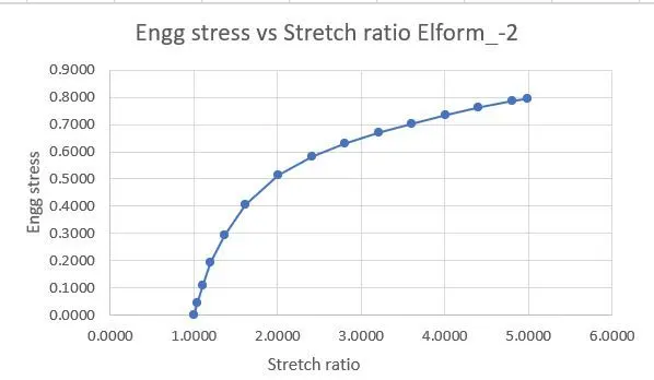
Engineering stress vs stretch ratio plot for Elform_-2

Engineering stress vs stretch ratio plot for Elform_2

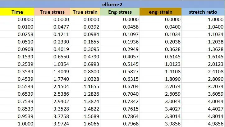
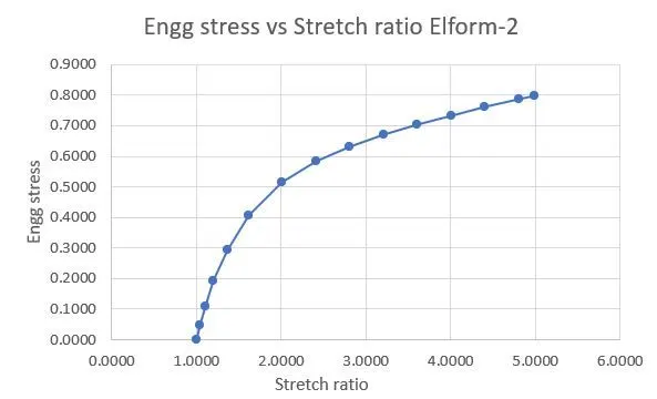
The graphs from the different cases were plotted for the Engg stress vs Stretch ratio. The maximum stresses were induced at 0.8Mpa for the stretch ratio of 5. The above all cases, the Stress values are almost the same. It shows that the stresses induced in the model are the same since the model and loading conditions are simple.

Conclusion:

The Fe model of a solid block with Odgen material was analyzed under slow steady loading conditions to simulate uniaxial tensile tests with different kinds of Elforms(1, 2, -1, -2). The Engineering stress/strain values and stretch ratio were calculated using some relations. Finally, Engineering stress vs stretch ratio values was used to plot the graph for getting output values.