Assignment 6-Frontal Crash Simulation Challenge

Objective:

To perform a frontal crash analysis on the BIW of the dodge neon car. To carry the crash analysis at the speed of 35 Mph. To generate the output requests are as follows

• Sectional force in the rails at the location of indicated node 174247.
• Axial force received on the rails from the bumper.
• Shotgun cross sectional forces.
• A pillar cross section.
• Acceleration curve received on the accelerometer at base of B pillar (on B pillar rocker).
• Intrusions on the dash wall 66695,66244.

Theory:

Crash analysis:

Overview:

Crash simulations are used to investigate the safety of the car occupants during impact on the front end structure of the car in a frontal impact, the lateral structure of the car in a side collision, the rear end structure of a car in a rear impact. Crash simulation can also be used to assess injury for the pedestrian. However, the main objectives can be given as-

• To ensure the safety of drivers.
• Selection of material on the basis of strength.
• Minimizing the weight of the vehicle without compromising safety.
• To reduce the cost for actual crash testing.
• The results can be used to assess both the crashworthiness of frames and to investigate the ways to improve the design.

Method:

Crash-testing requires a number of the test vehicle to be destroyed during the course of the tests and is also time consuming and uneconomical. One new recent trend that is gaining vast popularity is computer simulated crash-testing. Here instead of a real vehicle, a FE (Finite Element) model of the vehicle is generated and is used to carry out the different tests that were carried out before using actual vehicles.

Procedure:

Case setup:

In this project, We need to create a rigid wall, interface type 7 contact, check for penetrations, create initial velocity at 35mph, carry out mass balancing to ensure the body weight of 700 kgs & move the cog point to the correct area by adding mass under 700kgs. Finally create sections, accelerometers and intrusions for output request purposes to plot the graphs.

Here we use Hypermesh and hypercrash for pre-processing the model. Hyperview and hyper graph to generate animation and plot the graphs.

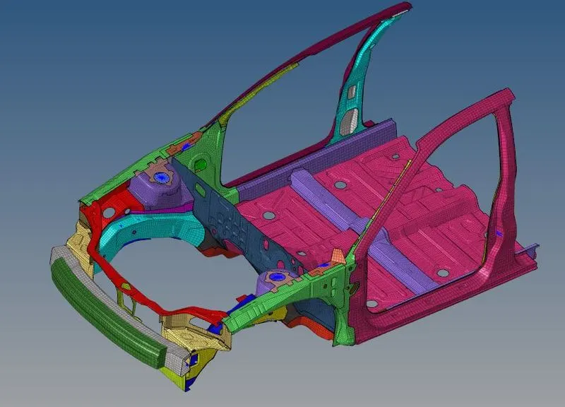
Model image:

Create type 7 contact:

Import the model using import>solver deck>.rad file and select import in hypermesh. Now the file is imported.

Check the units in Begin card>solver browser for kg,mm,ms.

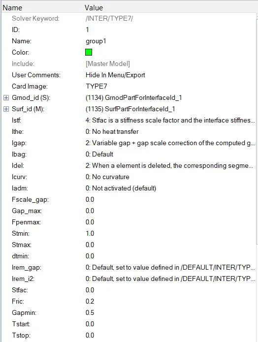
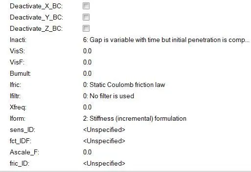
At first delete any type 7 contact that is already assigned. Now create>Inter>type 7. Here assign the recommended values for the type 7 contact. The image is shown below. Assign all components for slave and master node selection. Therefore the interface card covers all the components that are selected.

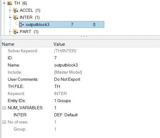
We need to create an output request for type 7 contact in time history. So select create>TH>Inter. After the interface attributes tab appears below, we need to right click entity id and assign a group that is created.

Creation of Rigid wall:

A rigid wall is an entity that is used to define an interaction between a non-deformable entity and deformable entity. Nothing can go beyond Rwall and it is non-yielding. It has multiple types like infinite plane, infinite cylinder, infinite sphere, infinite parallelogram. Here we should use infinite plane for frontal crash.

Next step is to create a Rwall for the crash analysis. At first create>Rigid wall>plane. Now select the node to create a plane at the centre of the bumper. Now assign Normal values for this x as-1, y & z as 0.

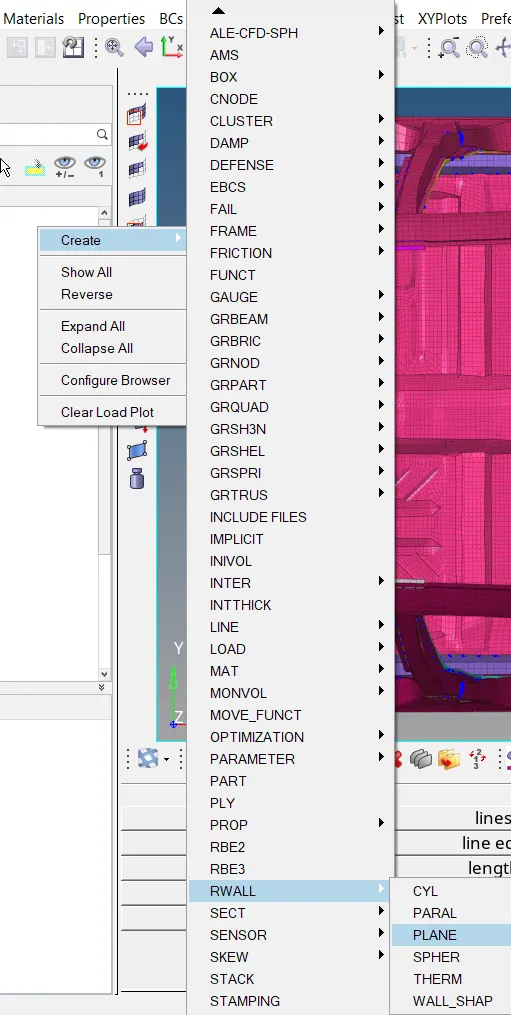
Now we need to assign Dsearch as 2000, Sliding as 2 (sliding friction), friction as 0.1. Assign nodes as all the nodes by box selection.

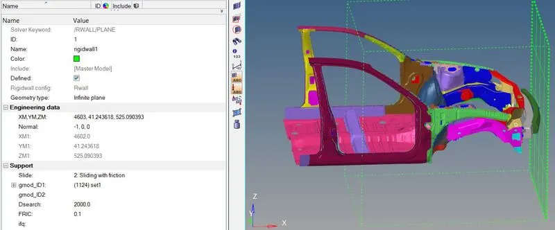
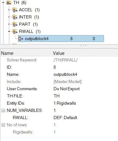
We need to create an output request for Rwall in time history. So select create>TH>Rigid wall. After the rigid wall attributes tab appears below, we need to right click entity id and assign a rigid wall that is created.

Assigning initial velocity for the model:

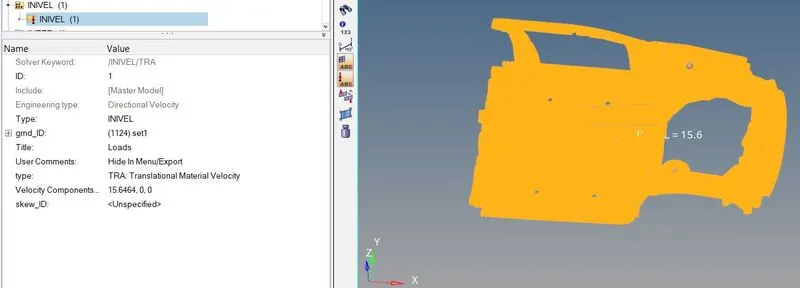
Now assign initial velocity for the car because here the car is the movable object not a rigid wall. Select create>Boundary conditions>INIVEL.

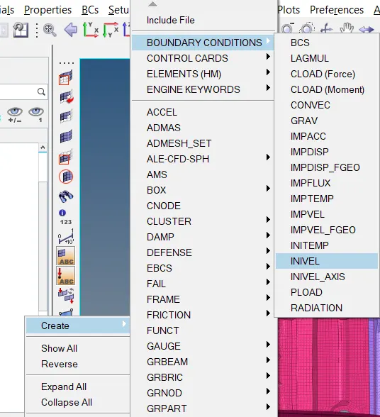
Here assign type as translational, Vx (x axis) velocity as 35mph. We need to convert miles per hour to mm per ms by converting the value to 15.64 mm/ms. Assign other two Vy,Vz as 0. Assign nodes and select all nodes for initial velocity.

Mass balancing:

Now export the model export>solver deck>.rad file. We need to import it to hypercrash for mass balancing. import>Radioss> .rad. Now the target mass of the model is 700 kgs. We need to check the mass of the model and place of the cog point by selecting Mass>Balancing from the toolbar of the hypercrash.

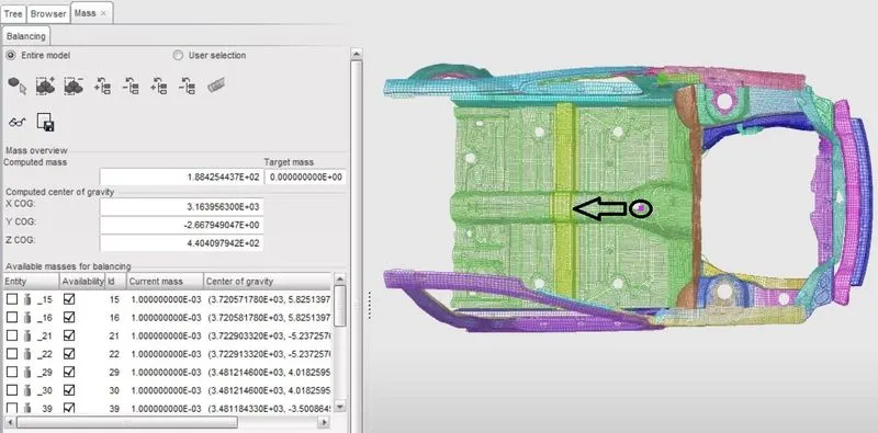
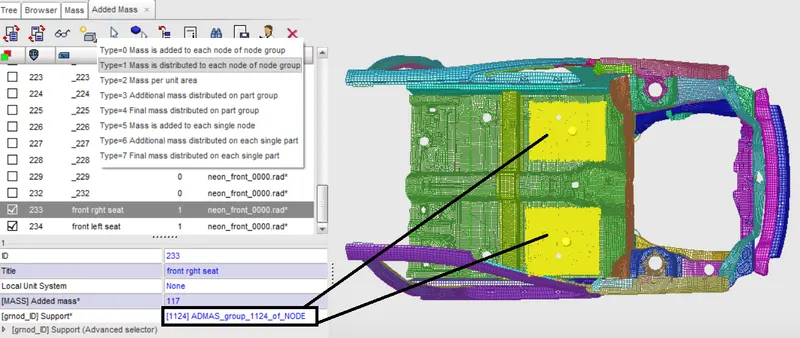
Here we have only 188kgs so we need to add some masses in the model to balance the mass in the overall model under 700 kgs.Centre of gravity point is shown above image. We need to move the cog point in the correct position by adding more mass and balance the weight to move the cog point. Now select Load case>Added mass. Select create a new object option and select type as type 1 for adding mass. Now assign the additional mass in kgs. Now select the node for adding the mass to those nodes. Here I need to select the front passenger seats floor separately. We can add masses at some other floor areas to balance the model.

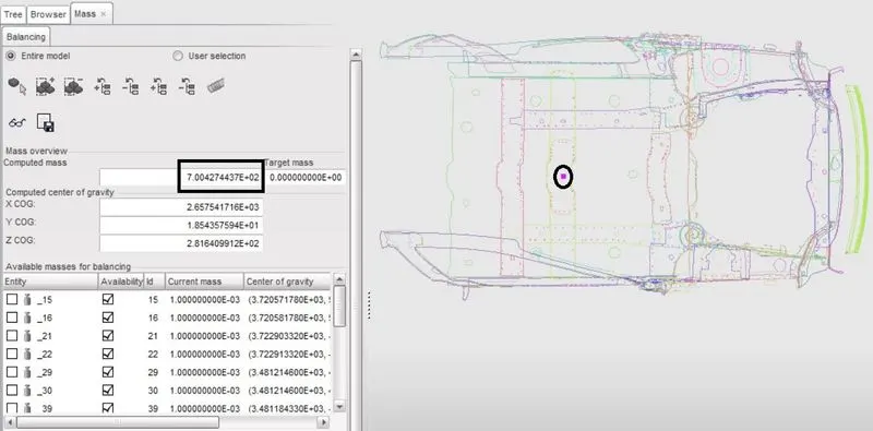
The following the current mass of the model and cog point where we want are shown below.

Output requests:

Creating sections:

At first creating sections we need to create a moving frame( local coordinate) for sections. Select create>Frame>mov to create frame.

Doing this the moving frame window appears on the screen. We need to select the origin node and select node for z axis & select node for yz plane. For the origin node, we have node id (174247) to select for rail sections. For this right click the origin node tab and select by id option, put the node id and select add to show up the node. Select the other two nodes to define the plane.

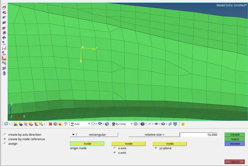
After creating a moving frame, we can create a section for the moving frame by selecting create>sect>sect.

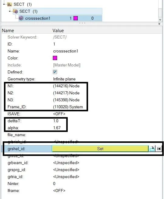
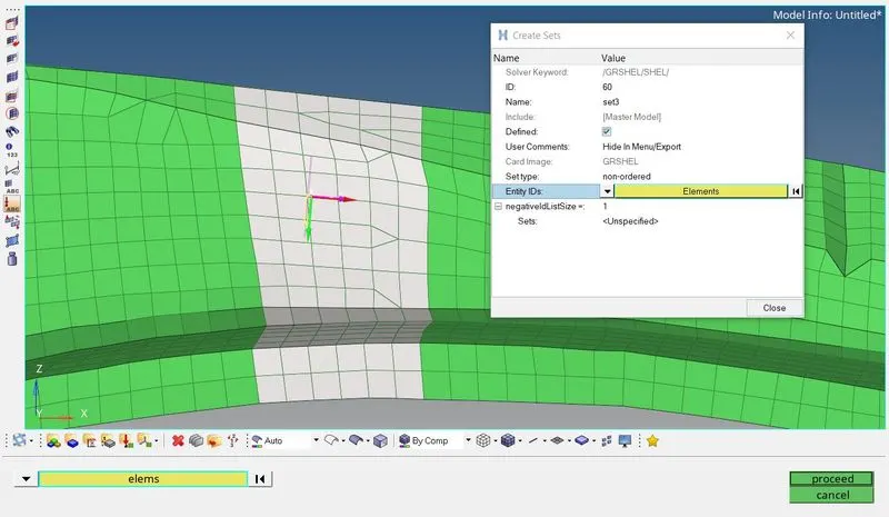
Now select N1 node is an origin node that is defined for a moving frame. N2 & N3 nodes are selected to define a plane. After this, select a frame id by selecting the frame that we already created. Put the Delta t as 0.1 and alpha value as 1.67. Now we need to select grshel_id. It will be selected by two rows of elements, of which the nodes are a part. Now check the arrow that would be perpendicular to the force acts or parallel to the Rigid wall.

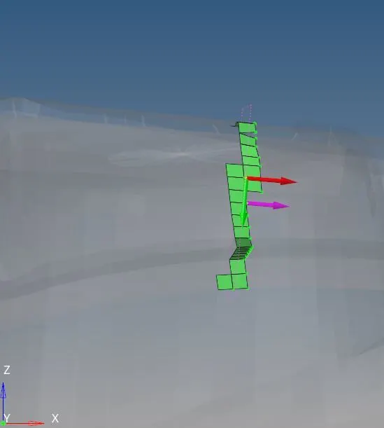
After creating the sections, we need to create output requests in time history by selecting create>TH>SEC. After this, right click out blocks. select entity ID and we need to assign all the sections that we created (8 sections).

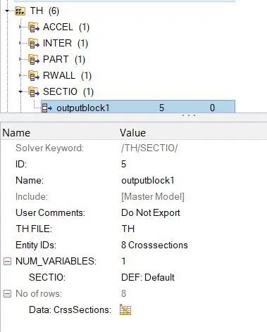
Screenshot will all cross sections that are created shown below.

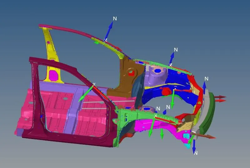
Creating Intrusions:

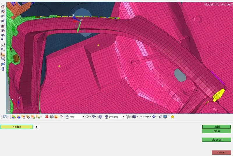
Here we have different kinds of methods for adding intrusions. But we go on using the spring element method. For this we need to add temp nodes or number the particular nodes(66695,66244). We go on adding temp nodes. Select geometry>temp node. Now right click node>by id (66695,66244). Here put the node id and click enter and then select add to create the node.

.

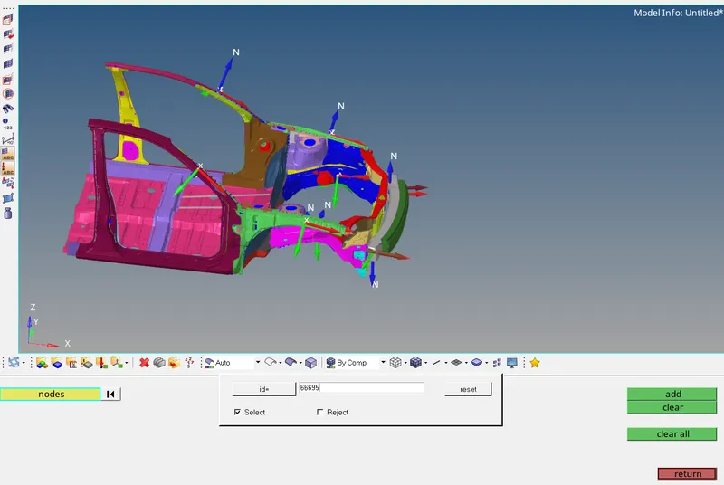After creating the temp node, we need to create a 1D spring element. Here select 1D>springs>two nodes. Now select the first node as temp node that is created already. Select the second node that is parallel to the temp node. Now select create.

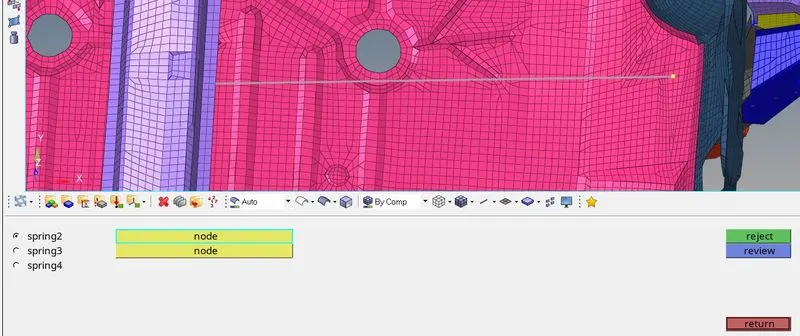
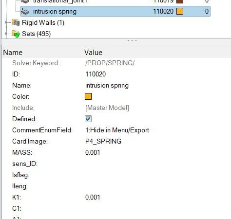
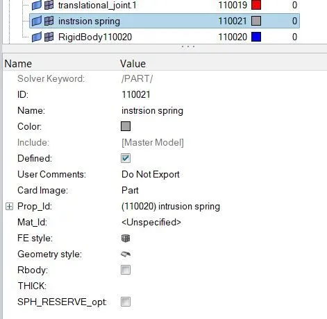
Now we need to rename it in model browser>components>undefined. Now create a property id for the spring element part. Assign mass as 0.001 and stiffness k1 as 0.001. After this, assign property id for the spring element part.

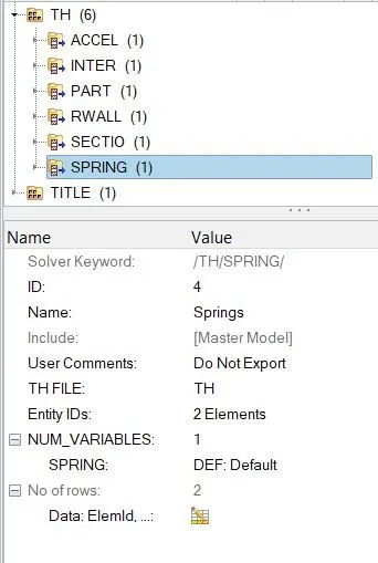
Now we need to create output requests in time history by selecting create>TH>Spring. Now select the entity id and assign two spring elements.

Creating accelerometers:

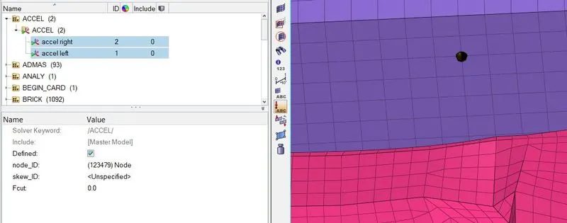
To create accelerometers, we need to go to model browser>right click>create>accel. Here we need to assign a node ( at the base of B pillars) in node ID.As we can see the node selected and marked as an accelerometer.

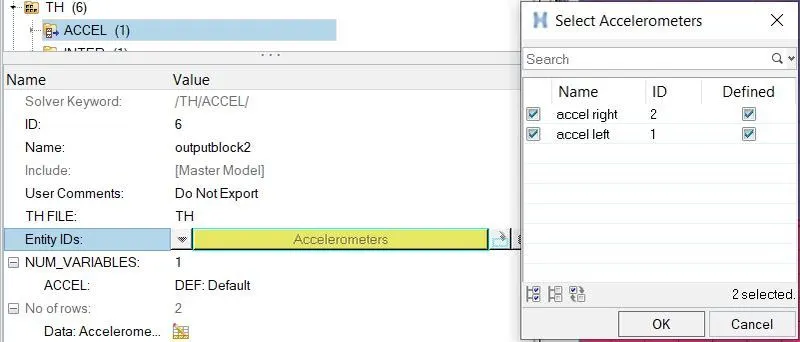
We need to create output requests in time history by selecting create>TH>accelerometer. We need to assign a created node in entity id. Follow the procedure right side entity also.

Penetration check:

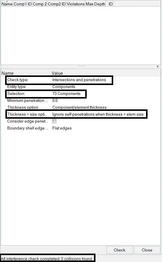
We need to check for any initial penetration in the model. For these select tools>penetration check on top of the tool bar. Now select the check type as intersections and penetrations. Entity type as components and assign all the components. Thickness>size option as ignore initial penetrations. Now select check for check the entities.

Check Simulation time:

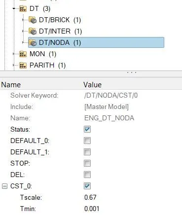
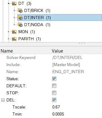
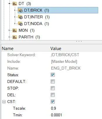
Go to solver browser>engine keywords>DT. Check Tmin in DT NODA, DT BRICK, DT INTER. Assign value as 0.1 to 0.5 micro seconds.

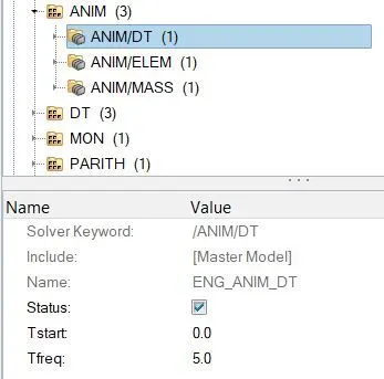
Go to solver browser>engine keywords>ANIM>ANIM/DT. Check Tfreq as 5.0.

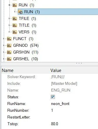
Go to solver browser>engine keywords>RUN. Check Tstop as 80ms.

Model checker for errors:

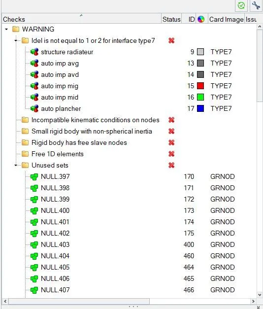
Finally we need checking for errors in the model before doing analysis. Go to tools>model checker> right click RUN.

Here we have warnings only so we can ignore the warnings. If any errors arise, we need to rectify the errors.

Running the model analysis in Radioss:

Now select the analysis section in the bottom panel. Here select Radioss.Here we have to save the simulation files by selecting save as tool. We should create a folder for saving analysis files separately. because we will get a lot more files after simulation. select the correct directory to save those files. After that choose export options as all, check the include connectors checkbox, type -nt 4 in options tab (it runs the solver using 4 cores on the CPU). Now select Radioss to run the simulation.

Analysing the output file:

The next question is to carry out the energy error and mass error in the simulation. So we need to go to the analysis saved files directory and open _0001.out file to check the error by using text editor. By opening the file, go to page down. We can see the energy and mass values for the end time step. The resultant energy error is -2.1% which is acceptable. The energy error is acceptable between -15% to 5%. The closer to 0% is better. The mass error is 0.001. It means the negilgible quantity of mass 0.001gram was added for the simulation possibly for control the time step. It was low amount so it is acceptable.

Viewing the simulation:

To view the simulation, we need to switch to hyperview by using a client selector.

Here we have to import the h3d file in the saved directory. After importing, select the contour tool in the toolbar. We can switch to von mises contour. We can analyze the model using this contour.

The animation is shown below,

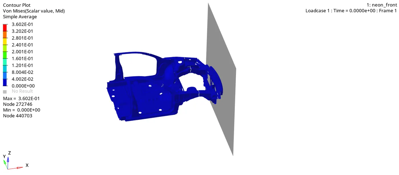
After the car BIW hits the rigid wall, The maximum stress is flowing from bumper through A pillar and floor panel. Maximum stress value is 0.360 Gpa at Node 272746.

Plotting the graphs:

Next we should plot the energy graphs and output request graphs using hypergraph 2D view. Go to the client selector, we can switch to hypergraph 2D. We should import the T01 file in the saved directory in the load files tab.

Select global variables and select internal, kinetic, total, hourglass, contact energy and select mag and click apply to plot the energy graphs.

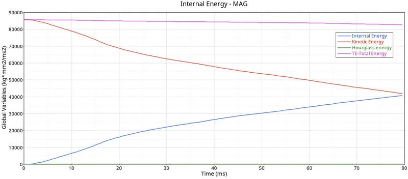
The above energy graph shows that the kinetic energy starts 80kJ high at 0ms after the car moves due to initial velocity at 35mph. After the crash, the kinetic energy drops to 41690J at 80ms. At the same time, the internal energy starts at 0 at 0ms. After the crash, the car absorbed the energy while hit the wall. the internal energy reached 4097J at 80ms. Due to the initial velocity of the car, The kinetic energy starts at high. after the car hit the wall, the velocity drops out the kinetic energy decreases gradually and got constant where the velocity of the car got constant. At the same time, the kinetic energy decreases. the internal energy starts at 0 and increases gradually due to the energy absorption while the car hitting the wall. The total energy is the sum of all the energy takes place. After constant, the total energy drops slightly due to contact energy. Hourglass energy is constant due to the presence of recommended shell properties.

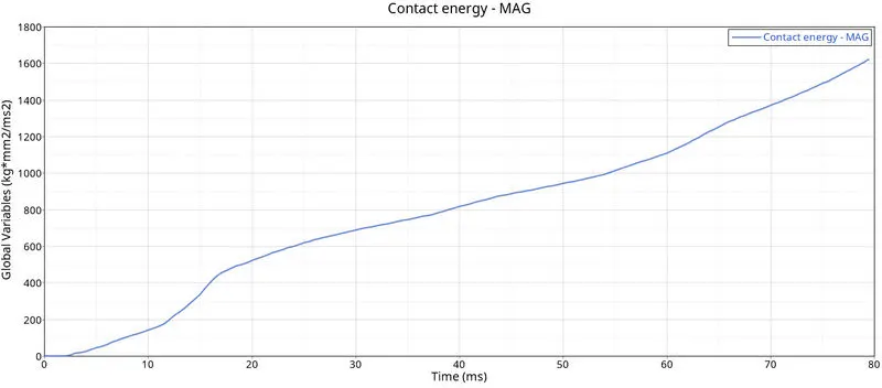
Contact energy starts 0 at 0ms. after the crash, the contact energy hit around 1650J at 80ms. Due to the elements got contact with other elements during crash, The element penetrations lead to increase in contact energy. The elements were penetrate with each other during the car hit the rigid wall. the elements got deformation and contact with other elements.

Rigid wall forces graph:

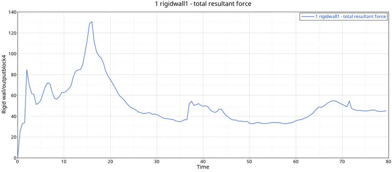
The rigid wall forces peaked at around 17ms when the car had exhausted its deformable capabilities in the bumper region. After that the forces were transferred to the other regions in the BIW. Due to that the rigid wall experienced the reduction curve during that time.

Output requests graph:

Cross sectional forces on both A pillars:

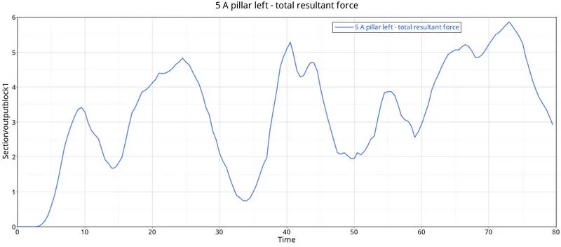
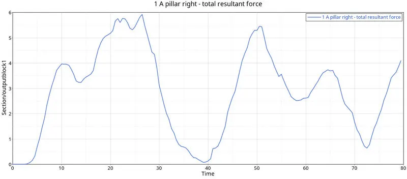
The maximum cross sectional force at left A pillar peaked at 73ms but the maximum cross sectional force at right A pillar peaked at 27ms. When the force was unevenly distributed through A pillars because the right side of the car deformed quickly over a time due to the centre point of the car being taken slightly to the right side of the car. Due to this, the forces were distributed unevenly through the car.

Cross sectional forces on shotgun members:

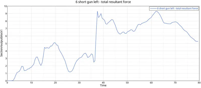
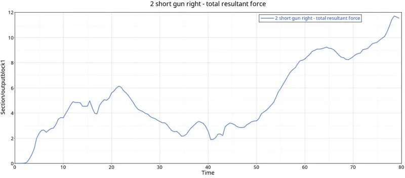
The left shotgun deformed first before the right side because of that the force of the left side peaked earlier at 37ms.The right side of the shotgun peaked at 78ms. But the right side got the maximum forces around 11.8 KN. The location of the sections may be non symmetrical due to this the forces were unevenly distributed through the members.

Axial forces on bumper rails:

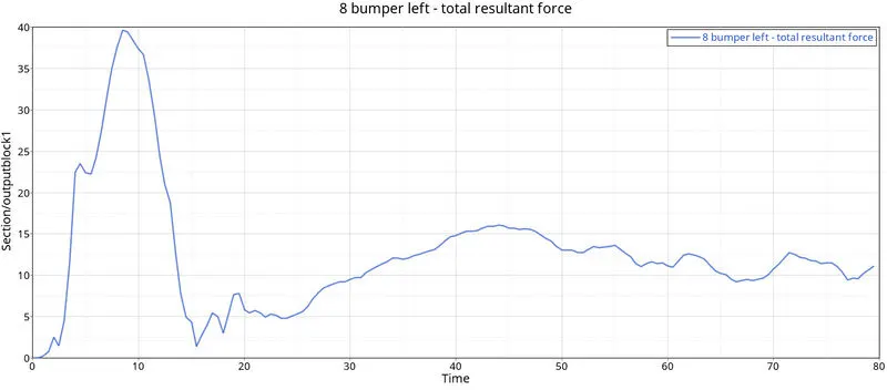
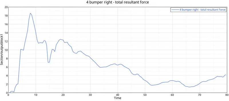
The Left side of the bumper peaked at 39 KN at 8ms. The right side of the bumper peaked at around 19 KN at the same time 18ms. Due to the location of the point was not symmetrical, the both sides of the bumper peaked at different maximum forces over the same time.

Sectional forces on both rails:

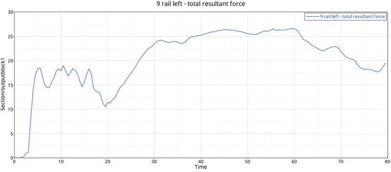
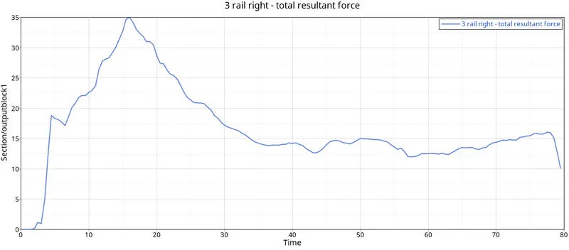
At first the left rail peaked around 27 KN at 60ms and dropped gradually over the time. The right rail peaked at maximum 35 KN at 17ms and dropped suddenly and got constant vibrations over the time.The left rail evenly buckled over the time. The right rail buckled suddenly and got constant.

Accelerometers in both B pillars:

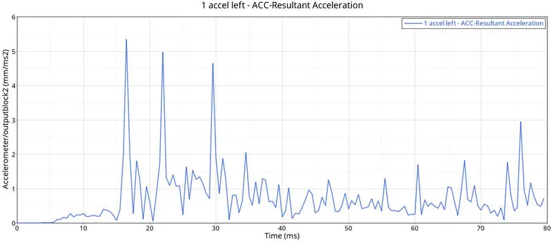
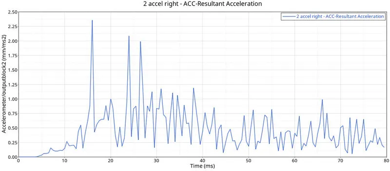
In accelerometer graphs, there were a lot of fluctuations over the time due to the vibrations over the BIW during the impact. The graph won’t spike when the BIW doesn't crash. It peaked at 2.35mm/ms^2 at 17ms.

Intrusions on the dash wall at 66695,66244:

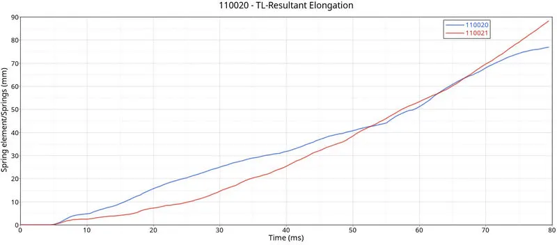
The Elongation of the spring peaked at 89mm and 79mm at 80ms. The good elongation length will be below 150mm. So the elongation of the spring at the two nodes was good at the crash.

Conclusion:

The front crash analysis was performed in the given dodge neon car model as per the requirements.The energy graphs were plotted as per the requirements. The output requests were generated using the sectional areas. Acceleration and the intrusions of the given nodes are also generated in the model.