Material Modeling from Raw Data

Aim:

• To use the diagram of the true stress-strain curve of graphite iron casting. Create material modeling for the given dogbone specimen using MAT_24 and validate it.

Objective:

• Extract the data from the diagram
• Clean the data and visually confirm that it matches the original data and the elastic modulus is 20.9E+06 psi.
• Convert the data to (kg-mm-ms) unit system
• Process the data and create the material as demonstrated
• Use the material model with a dogbone specimen and validate the same.

Procedure:

Here we have an image of the stress-strain curve of graphite iron. We need to extract the data points from the image using the "get data graph digitizer" application. We should use the set scale tool to define Xmin, Xmax, Ymin, and Ymax values. After that use a point capture tool to extract the points in the curve. Here we use curve-2 for getting data points for further use. Here we need to extract maximum points from the curve because LS-Dyna does not up to consider elastic limit. So we need to pick more points above 100. it is useful to get the Non-linear region more precisely.

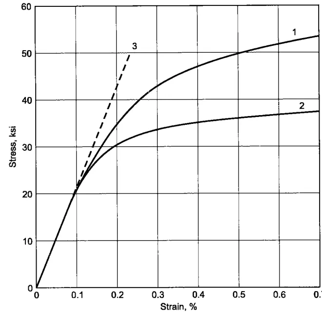
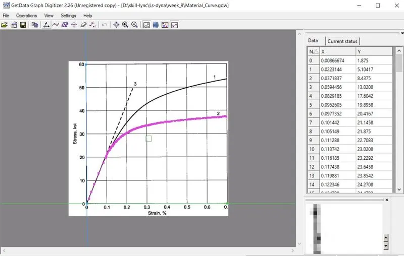
Obtained data points are in the form of Engineering strain and stress. We need to convert the true stress and strain. after that convert the true stress-strain values into effective stress & plastic strain values.

• True stress=(eng stress)*(1+eng strain)
• True strain= ln(1+eng strain)
• Effective stress=true stress
• effective plastic strain=total true strain-(true stress/E)

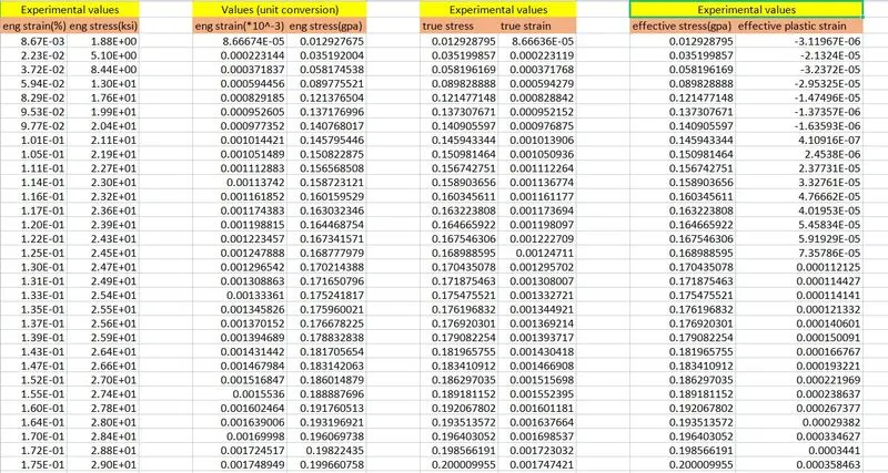
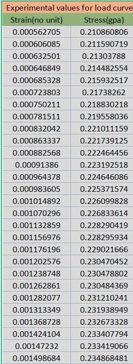
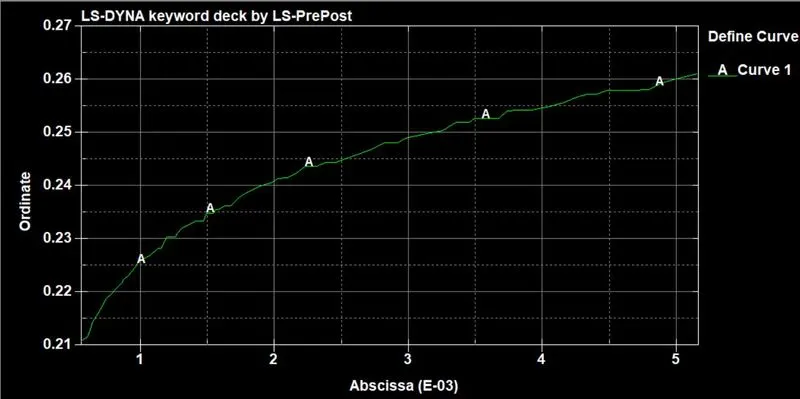
Here we need to extract the effective stress-strain points from yield stress 0.2. we need to take the values after yield stress(0.2) for plotting load curve in MAT_24. Here we need to remove the negative slope values to avoid negative slope error using slope formula=(y2-y1)/(x2-x1).

After that, we have the effective stress-strain values from the non-linear region(after yield stress).

Now we need to define keywords for the simulation.

Open the model using the open>keyword. The given dog-bone model is opened.

Here we need to give some keywords as follows,

Defining section card:

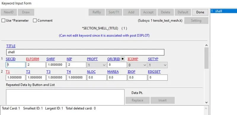
Go to model&keywords>all>section>shell. here we need to define sec id-1, Elform-2, thickness-1mm. Now accept and done.

Defining Curve:

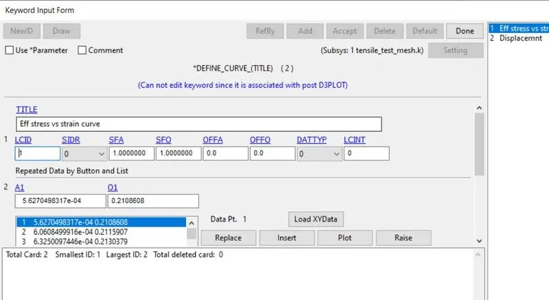
Go to model&keywords>define>curve. now define LCID-1. define data points using the load xy tab. now select the effective stress-strain values from the non-linear region(after yield stress).now select accept and done.

Defining MAT_24 material card:

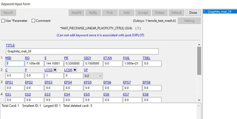
Go to model&keywords>all>MAT>MAT_24(piecewise_linear plasticity). now define ID-1, RO value, E value, Poisson's ratio, SIGY and define curve id-1. Now accept and done.

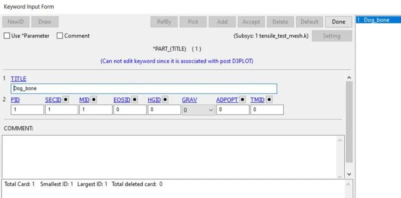
Defining part:

Go to model&keywords>all>part. define sec id, mat id. now select accept and done.

Defining boundary conditions:

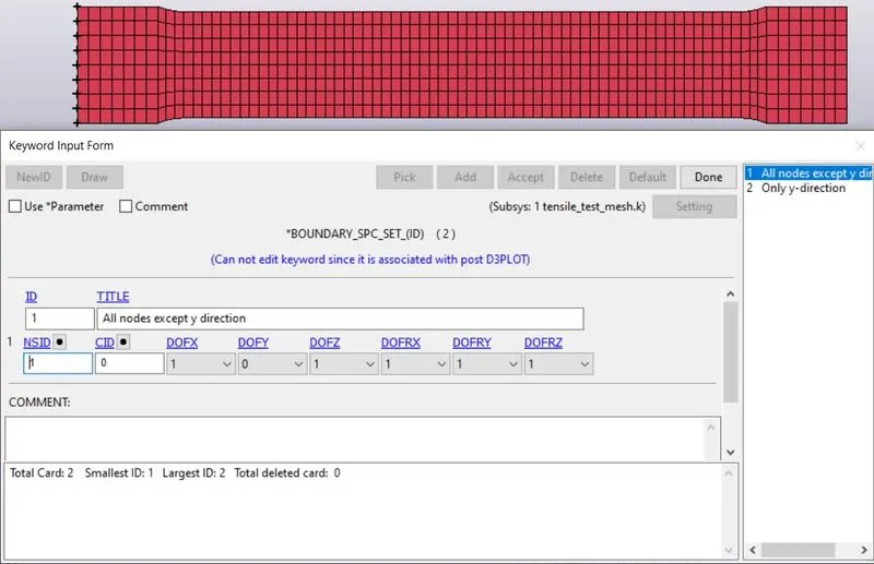
First, we need to create set_node to define boundary conditions. Go to model&keywords>create>set_node. Select nodes and select apply and done.

Now define Boundary conditions using model&keywords>all>Boundary>spc_set. Now define id number, node-set id, select all dof's as 1 except y-axis.

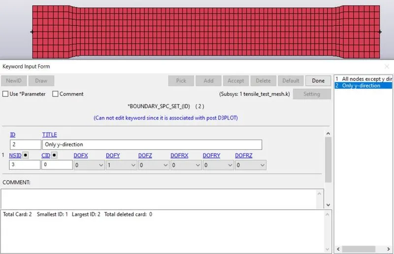
Go to model&keywords>all>Boundary>spc_set. Now define id number, node-set id, select only y-axis as 1.

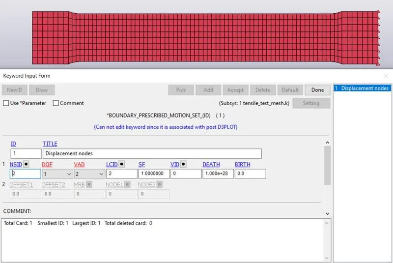
Now define displacement nodes for node-set. Go to model&keywords>all>Boundary>Prescribed_motion_set. Now define id number, node-set id, select DOF as 1(only x-axis), VAD as 2(for displacement), LCID as 2(for define displacement curve).

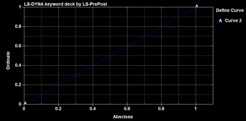
Defining curve using Go to model&keywords>define>curve. now define LCID-2. define data points using the insert tab. now put values. now select accept and done.

Defining database:

Define ASCII using model&keywords>all>Database>ASCII. now define GLSAT, MATSUM as 0.01. Now apply and done.

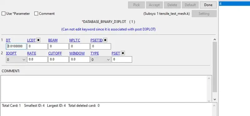
Define Binary d3plot using model&keywords>all>Database>Binary d3plot. now define DT as 0.01. Now apply and done.

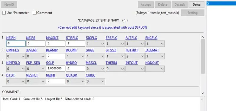
Define Extent_binary using model&keywords>all>Database>Extent_binary. now define STRFLAG as 1. Now apply and done.

Defining control card:

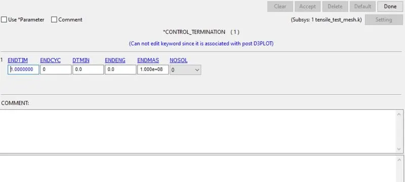
Define control termination using model&keywords>all>Control>termination. Define Endtime as 1.

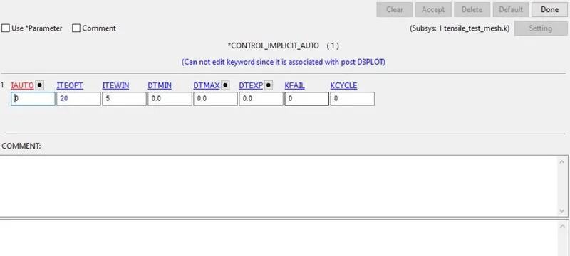
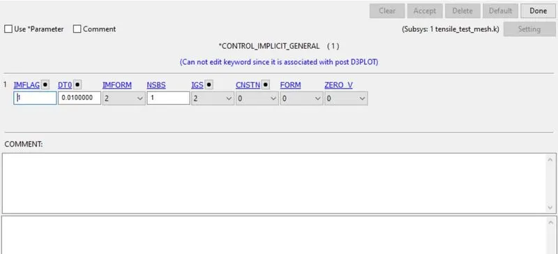
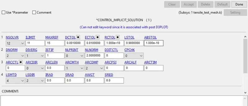
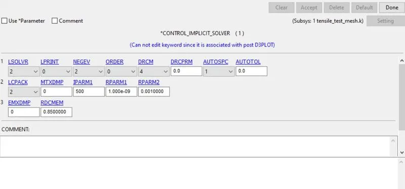
Here we should do implicit analysis for the model. so that we need to give implicit control cards using model&keywords>all>Control>implicit cards.

Implicit_auto:

implicit_general:

implicit_solution:

implicit_solver:

Results:

effective stress:

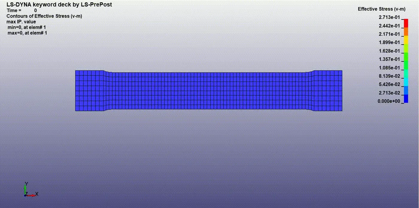
The maximum stress was induced at 2.7e-1 gpa.

effective plastic strain:

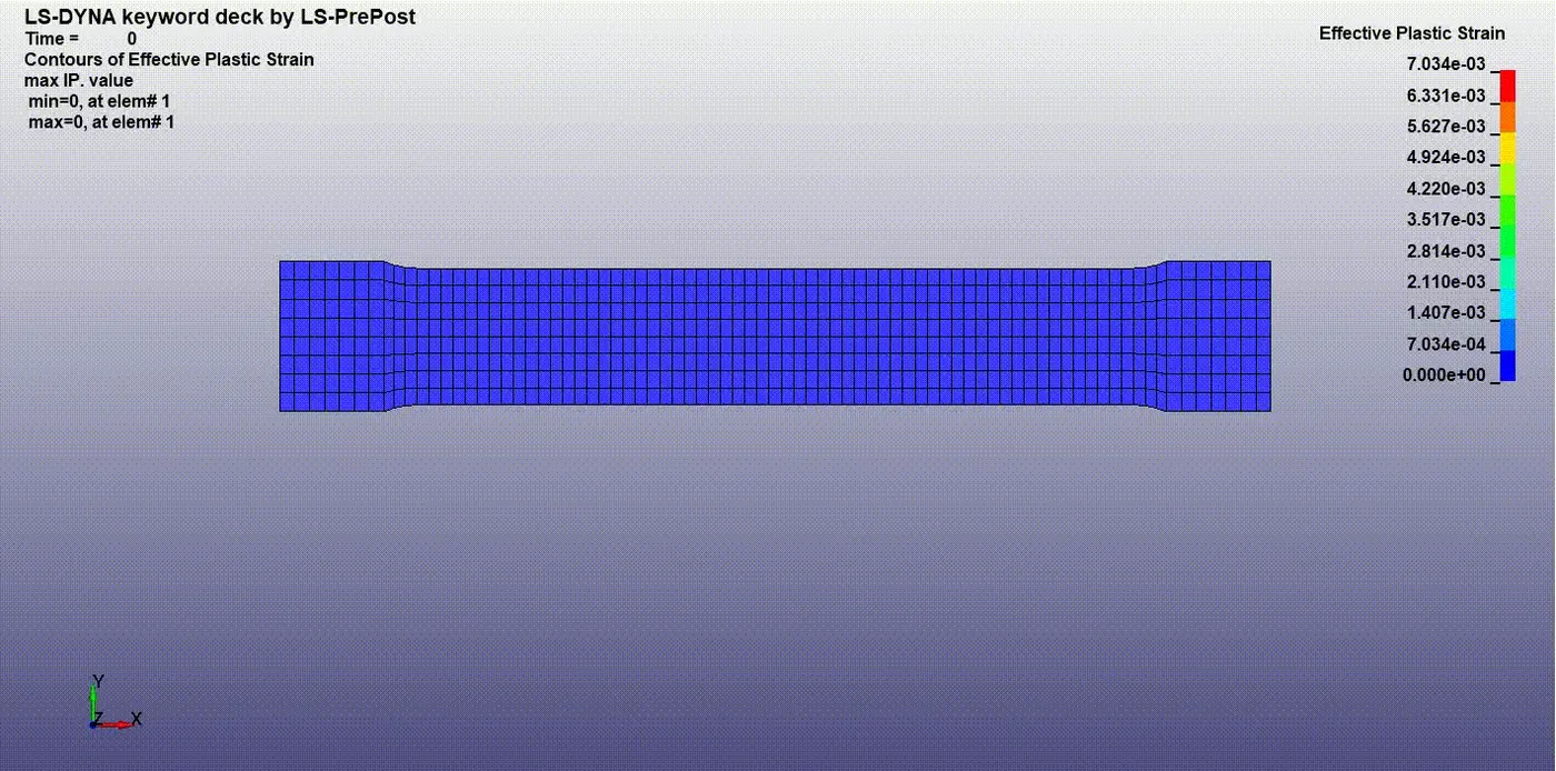
The maximum strain was induced at 7e-3.

Effective stress vs Plastic strain graph:

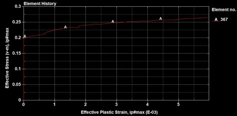
The plastic strain curve starts at 0.2 above because we define load curve after the elastic limit. so that the curve deviates after the yield stress 0.2.

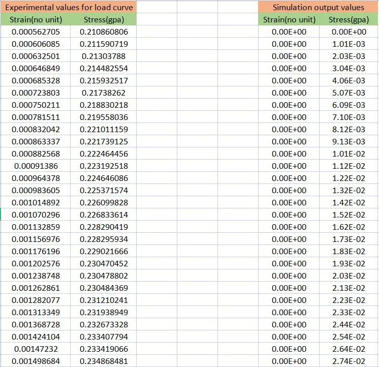
Experimental values vs simulation result values graph:

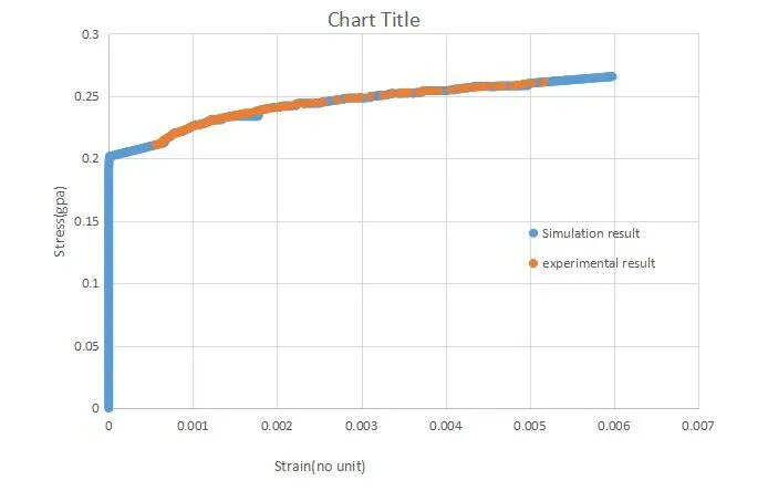
Here we can see both the curve from simulation output values and experimental values are more or less the same in the non-linear region.

Conclusion:

• Data capturing from the image for the material modeling was very precisely done.
• MAT_24 was defined for the model using an effective stress-strain curve derived from a given image.
• Compared both simulation results and experimental data.