Assignment 5-RADIOSS Interfaces & Study of Effect of Notches Challenge

objective:

1. To mesh the given bumper assembly with target mesh element size of 6mm.
2. To do simulations on a given crush tube model using various cases as follows.

• Run the crash tube model as it is.
• Change the Inacti=6 and run.
• Create the type 11 contact and run.
• Remove both notches and remove boundary condition on rigid body node then run.
• Create a new notch in the middle ,select the whole section and run.
• Create a new notch with nodes only from opposing 2 faces and run.

3. To plot the RWALL forces and Energy graphs for various cases and compare the results.

Theory:

Interface/contact modeling:

The interface modeling is defined as how the parts get contact with each other. Explicit analysis solves highly complex non linear problems and contact plays important role. The interfaces are defined through master segment and slave nodes.

The algorithm takes master segment and slave nodes and check for initial penerations between master and slave nodes for every time step.

Most widely used algorithms are

• Type 7, variable stiffness, node to surface contact.
• Type 11, variable stiffness, edge to edge contact.
• Type 24, linear stiffness, node to surface & surface to surface contact.
• Type 19, combination of both type 7 & type 11 contact.

Penalty method:

1. The variable stiffness is because Radioss follows contact theory called penalty method calculation.
2. The penalty method is treating the master and slave segment as springs that resistive forces as a function of penetration.
3. An imaginary spring element is created between master and slave segments. The stiffness is based on the material property of the model.
4. time step is inversely proportional to stiffness.
5. They are two types of time step as nodel time step and kinematic time step. The simulation is governed by kinematic time step.

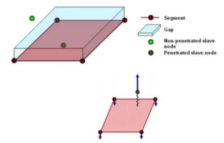
Type 7, variable stiffness, Node to surface contact:

Type 7 is a node to surface contact. it is a universal type of contact. A gap is defined between master and slave segment. The gap is constant or variable. The slave node is kept outside of the master gap by the resistive forces when the slave node enters into the master gap. the type 7 interface is non-oriented. slave nodes can belongs to the master segment.

Advantages of type 7:

• Physical correct representation.
• High accuracy for describing self contact and buckling.
• Best used with shells to shells and shells to solids.

Disadvantages of type 7:

• Require more stringent modeling practices.
• Does not tolerate intersections (slave node passing master segment)
• time step may reduce due to increasing interface stiffness.

Important parameters of type 7 contact:

we have to assign these 7 parameters when we create type 7 contact,

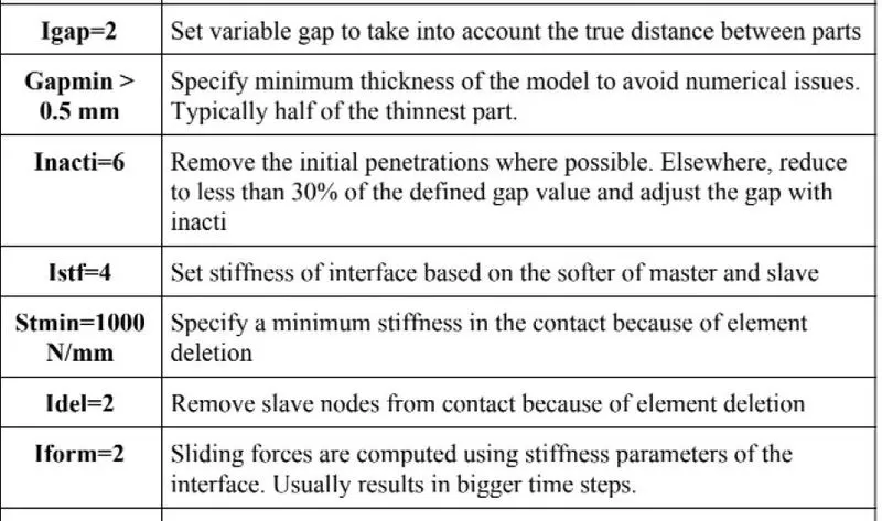
Igap- Dtermines how the size of the gap is calculated

Gapmin- Minimum gao for activation of interface.

Inacti- Action to take if initial penetration exist

Istf- Affects how the stiffness of the interface is calculated.

Iform- Friction formulation

St min- minimum stiffness to use in the interface.

Idel- What to do with slave nodes & master segment if the element fails (deleted) that they are attached to.

Igap- gap type:

Igap	gap type	description
0	constant	the gap is defined by Gap min and is constant for all the contact.
1	variable	Gap varies according to the impacted master surface and impacted slave nide.
2	variable	variable gap with gap scale factor
3	variable	variable gap with gap scale factor and mesh size correction

Recommended Igap value is 3.

Most widely used Igap value is 3 because the f-scale factor and mesh correction takes place to do simulation properly without failure. In Earlier when the components are at rest it may have initial penetration due to cloase contact. While F-scale factor is added that the factor relax the initial contact and which allows the slave node to reach the master segment easliy. If the mesh size is big, instead of slave node, the edge of the slave segment is contact with master segment. So the mesh correction factor allows to overcome this issue.

Inacti- Removing initial penetrations:

Initial penetration is defined as some slave nodes are already pass or penetrate the master segment when model at rest which causes simulation failure. This can be fix by this algorithm. while the algorithm is activated, some resisitive force act on the penetrated node to push out the slave node to disengage the node from master segment. The recommended value is 6.

Inacti	action	remark
0	no action	best option if possible
1	deactivation of node stiffness	low accuracy
2	deactivation of master stiffness	low accuracy
3	automatic removel of initial penetration	danger to use, may destroy the model
5	the gap is reduced	good accuracy
6	the gap is reduced & scaled	good accuracy

We choose Inacti is 6 because the gap is reduced and scaled. The solver removes the penetration and moves nodes 30% of initial penetration (p0) to avoid contact stability issues.

Istf-Initial contact stiffness:

Before getting into initial contact stiffness, we need to know about how the resistive force is calculated.the resistive force is calculated by taking the penetration of slave node into gap and is a function of penetration value and rate.

F=K*P+C(dP/dT) where K=K0*gap/gap-P and C=vis*`root`2KM. now to calculate the stiffness Kt=K*Gap^2/(Gap-P)^2.

Istf	initial contact stiffness
0	K0=Km
1	K0=Stfac
2	K0=(Km+Ks)/2
3	K0=Max(Km,Ks)
4	K0=Min(Km,Ks)
5	K0=(Km*Ks)/(Km+Ks)

Recommended value is 4. K0=Min(Km,Ks). Because of minimum stiffness, the resistive forces that are applied on the slave node will be kept to minimum.

Iform- sliding force computation:

Iform	formulation	description
1	viscous	sliding forces are computed using viscous parameters of the interface
2	stiffness	sliding forces are computed using stiffnes parameters of the interface. usually results in bigger time step.

Recommend value is 2. because the sliding forces are computed by stiffness parameters of the interface.

Idel:

This value indicates the update for deleted elements due to failure. the recommended value is 2.

Idel	action
0	No update:the master segment and free nodes are kept and may lead to instability
1	The master segment is removed from the contact when all the linked elements are deleted and slave nodes which becomes free are removed from contact.
2	The master segment is removed from the contact when one the linked elements are deleted and slave nodes which becomes free are removed from contact.

Finally the recommended parameters are as follows

Type 11- edge to edge contact:

One of the drawbacks of type 7 contact is that it cannot remove the element intersection that is present in the model. To avoid this kind of issue and edge related intersections, type 11 contact is preferred. type 11 works very much similar to that of type 7 but the search is for only the edge of the model.

Here the master and slaves are the component's edge lines.

• To detemine the contact forces, one can go to cards>ANIM/CONT.
• To detemine the contact pressures, one can go to cards>ANIM/PCONT.

The recommended parameters are the same as that of the type 7 interface. Always the more stiffer component is meshed with a coarser mesh than the slave component which is taken as master.

Procedure:

Meshing the bumper assembly:

After importing the model. we need to do geometry cleanup for the model using geometry> quick edit and geometry> surface edit tool.

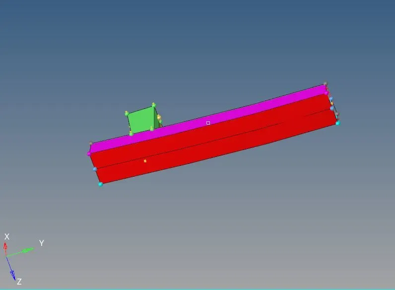
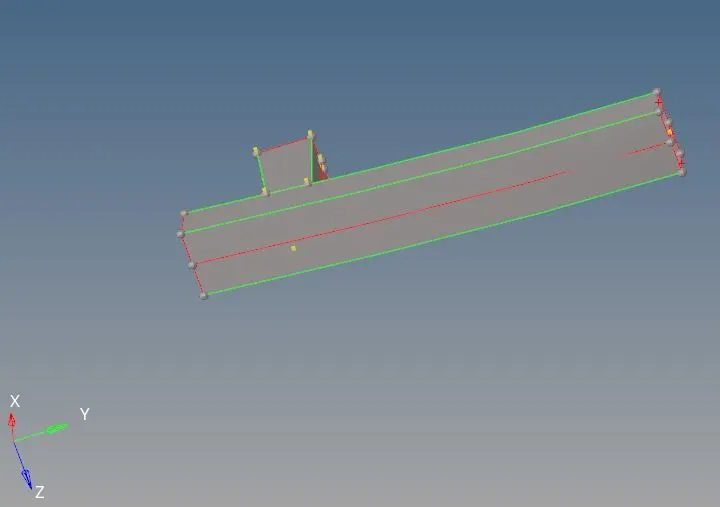
Use surface edit tool, select the extend option and extend the both edges of the surfaces to the target surfaces. Now the surface is extended.

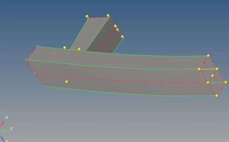
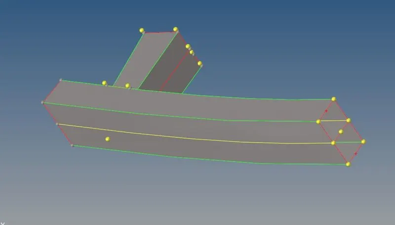
Use surface edit tool, select extend and extend the small surface to the target surfaces and now after extension, trim the extend surface by target surface and use quick edit to delete the surface which is extended irregularly.

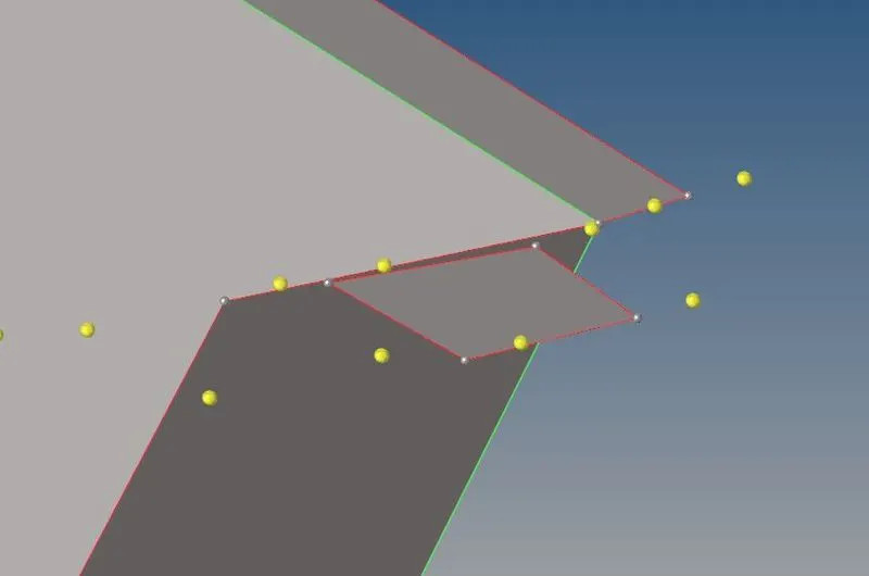
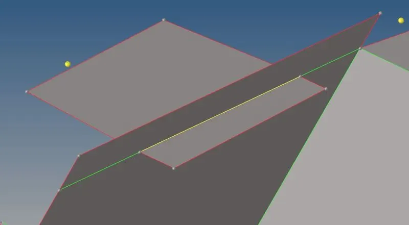
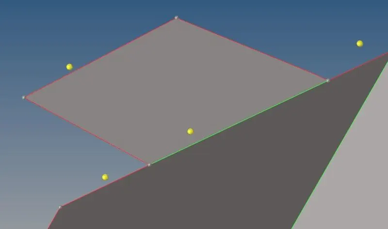
After the geometry cleanup, we can move to mesh the component. Go to 2D>automeshand select the surfaces to meshing and assign target mesh size as 6mm. now select mesh type as mixed.select mesh.

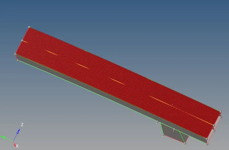
Now the entire component is meshed and the rotating quads and opposite & back to back trias are removed. The mesh flow is good.

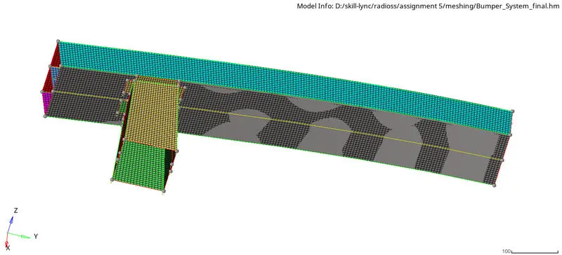
Running simulations on the crush tube:

Case 1: Run the crash tube model as it is & create interface in TH.

Import the crush tube file(0000.rad) via file>import>solver deck tool.

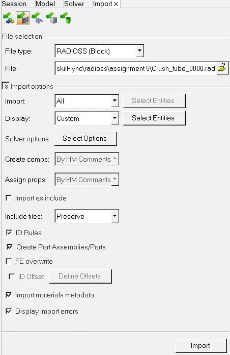
After importing the model will be shown below,

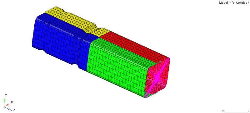
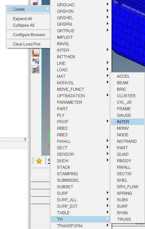
As mentioned in the question the output should be interfaces or contact forces. so we need to create interface in TH. So right click on the browser panel and select create>TH>INTER.

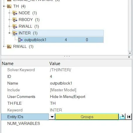
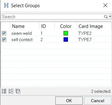
After creating Interface in TH. Now assign the groups of interfaces already created in the TH. Now run the simulation without change anything further.

After that run the simulation using analysis>radioss. select save as to save simulation files in some particular directory. and type -nt 4 in option tab for speed up the processors to run the simulation.

A few seconds later, the solver window pops up and run the simulation. after completion the results are shown as .text file.

Now open the 0000.out file in file directory to check the energy errors, no.of.cycles and elapsed time in the simulation file.

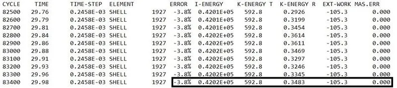
As We can see the energy error is -3.8% and it is acceptable since it is below -15%. there is no mass error (0%)

The next step is to view the animation by selecting hyperview in client selector. After that load the .h3d file.

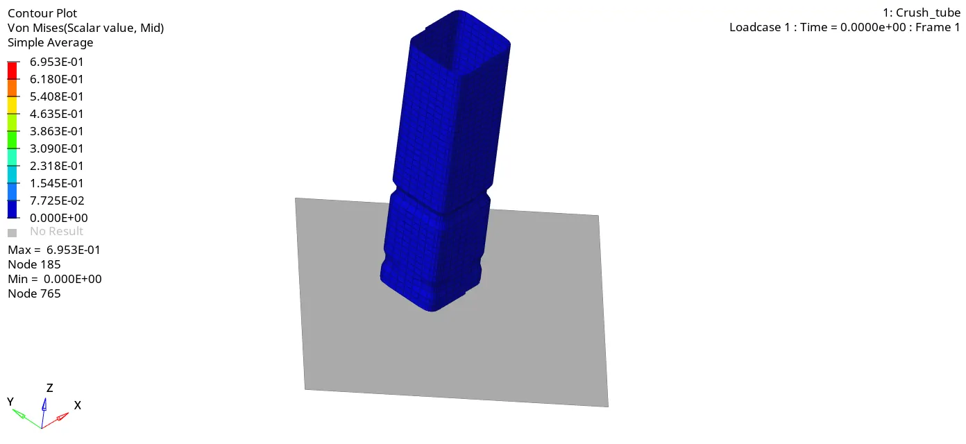
To run the animation,the contour panel should be selected. after that select parameters such as result type as von mises, selection as components, averaging method as simple and then select apply to run the animation.It is evident that the presence of notch that leads to stress concentration in those region. so the buckling occurs first. This will happen in all the cases which involving notches.

The simulation shown below,

Here we can switch to hypergraph 2D panel for plotting graph via client selector. In this panel, we need to load T01 file in file directory. Now select variable as Internal Energy, Kinetic Energy, total energy, contact energy, hourglass energy and select parameter as MAG and apply for plotting the graph.

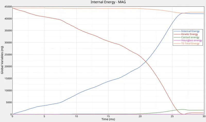
Internal energy keeps increasing due to the tube continuously absorbing energy while crash on rigid wall which results in deformation. when the deformation compltes the internal energy goes constant.

Kinetic energy keeps decreasing due to initial velocity on the tube. the curve starts from high values and decreasing to low due to the deformation. There is slight increase afterwards due to rebound after deformation.

Contact energy is a type of energy that is created when one element contact with neighbouring elements. The opposing force created by the element called contact energy. There is no contact in initial stage, so thats why the graph goes constant. At somepoint, the graphs slightly increases due to the buckling of elements.while the entire tube pressing on rigid wall, the buckled elements are forced into contact.

Total energy decreases at somepoint due to increasing of contact energy at the same time. so the contact energy affects the total energy.

Hourglass energy is constant due to the presence of recommended properties.

Now next step is to plot rigid wall resultant force graph for case 1 simulation, so select variable as rigid wall and parameter as resultant force and apply to plot the graph.

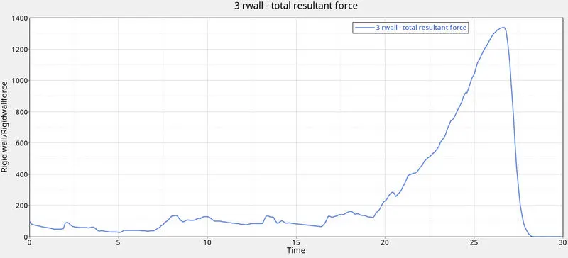
It is evident that the rigid wall experiences some forces immediately due to the crush tube crash over the rigid wall and absorb the energy from crush tube. after the deformation completes, the rigid wall force is decreased immediately due to the energy transferred completely.

Case 2:Change the Inacti=6 and run.

Import the 0000.rad file using import>solverdeck tool. Now change the parameter Inacti as 6 in inerface card. After that run the simulation using analysis>radioss. Follow the procedure as mentioned in case 1.

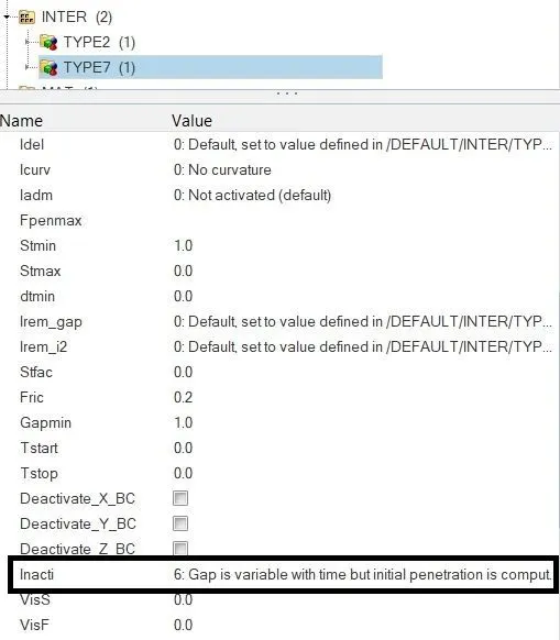
Now open the 0000.out file in file directory to check the energy errors, no.of.cycles and elapsed time in the simulation file.

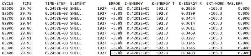
As We can see the energy error is -3.8% and it is acceptable since it is below -15%. there is no mass error (0%)

Now run the animation by selecting hyperview in client selector. After that load the .h3d file.

To run the animation,the contour panel should be selected. after that select parameters such as result type as von mises, selection as components, averaging method as simple and then select apply to run the animation.

the animation shown below,

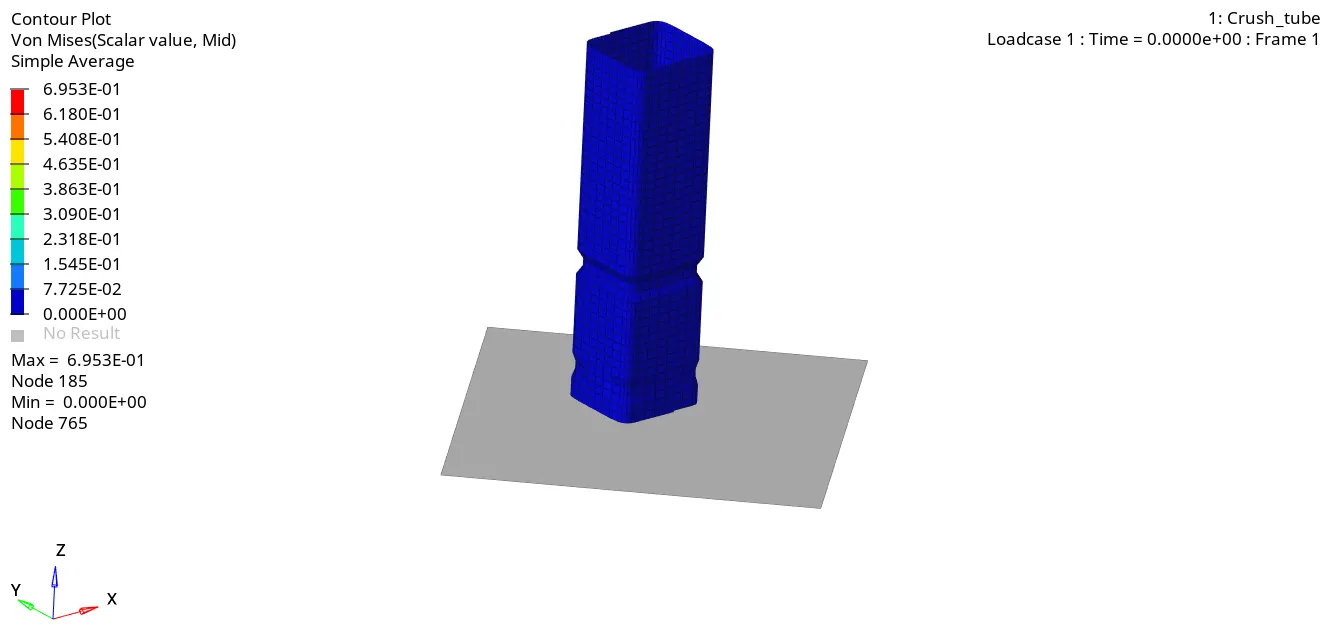
There is no evident differnece between case 1 and case 2 animations. They both are very similar. Even though the Inacti parameter is changed, it doesn't make any big difference. There was no initial penetration occurs due to Inacti parameter.

we need to switch to hypergraph 2D panel for plotting graph via client selector. In this panel, we need to load T01 file in file directory. Now select variable as Internal Energy, Kinetic Energy, total energy, contact energy, hourglass energy and select parameter as MAG and apply for plotting the graph.

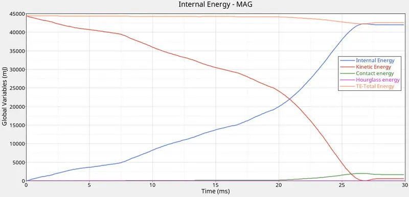
The energy graphs are similar between Case 1 and case 2 graphs. In contact energy shows same as case 1 even though Inacti parameter was changed because there is no initial penetration occurs. if there any penetration takes place, the contact energy starts at non zero value.

Next step is to plot rigid wall resultant force graph for case 2 simulation, so select variable as rigid wall and parameter as resultant force and apply to plot the graph.

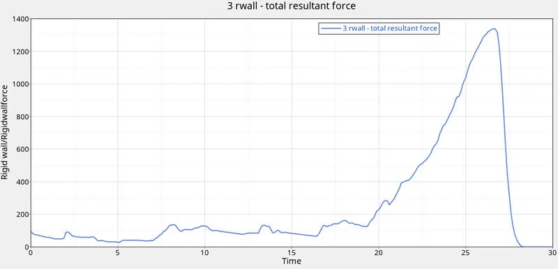
It is evident that the Rwall force also similar like case 1.

Case 3: Create the type 11 contact and run.

In this case, We need to create type 11 contact. For this right click at solver browser, create>INTER>type 11. We need to assign some parameters as shown below,

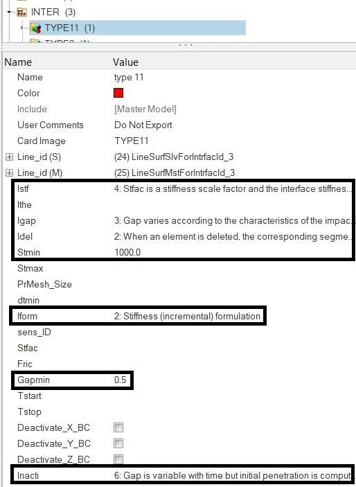
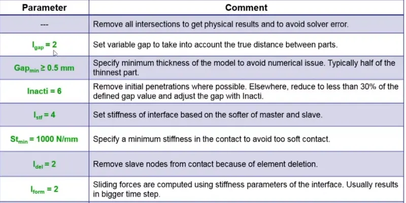
After creating type 11 contact, assign master and slave segment, assign all the components as master and as well as slave segment.

After this, Include type 11 contact as a group in TH interface.

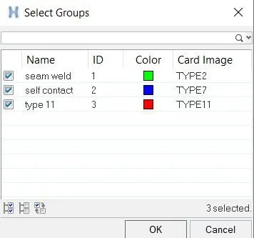
After all this, run the simulation as follow the procedure in case 1.

Now open the 0000.out file in file directory to check the energy errors, no.of.cycles and elapsed time in the simulation file.

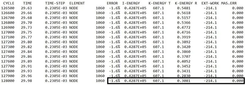
As We can see the energy error is -1.6% and it is acceptable since it is below -15%. there is no mass error (0%).

The next step is to run the animation by selecting hyperview in client selector. After that load the .h3d file.

To run the animation,the contour panel should be selected. after that select parameters such as result type as von mises, selection as components, averaging method as simple and then select apply to run the animation.

the animation shown below,

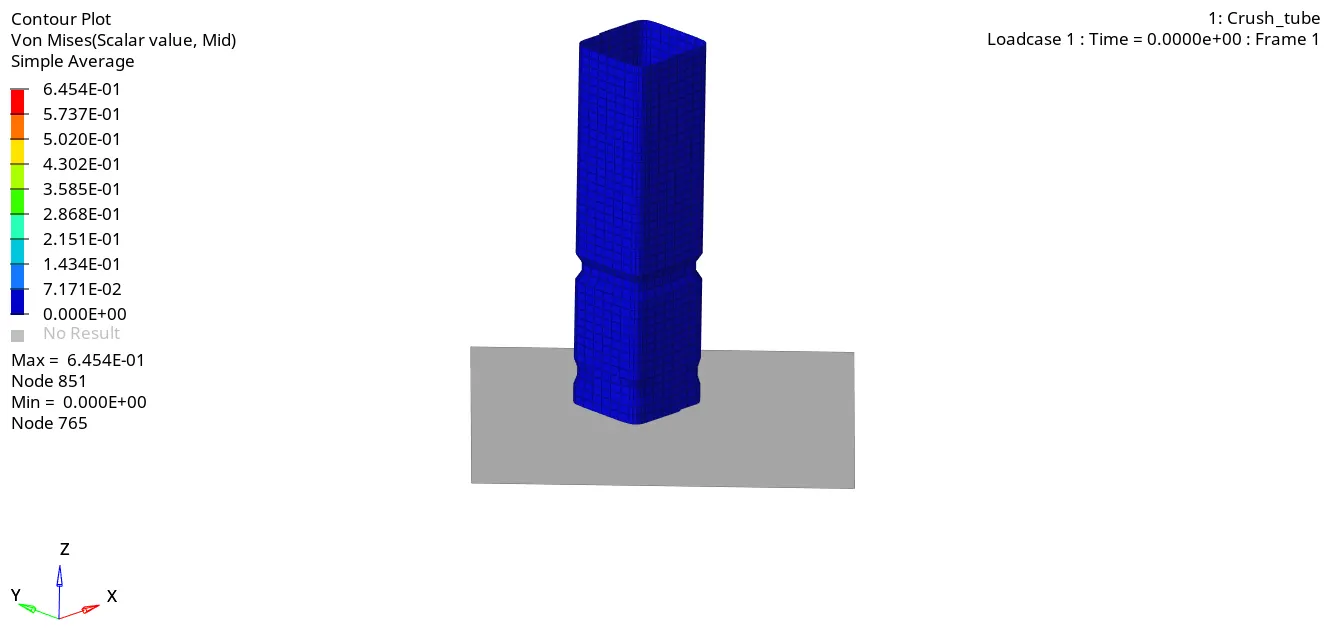
we need to switch to hypergraph 2D panel for plotting graph via client selector. In this panel, we need to load T01 file in file directory. Now select variable as Internal Energy, Kinetic Energy, total energy, contact energy, hourglass energy and select parameter as MAG and apply for plotting the graph and Next plot rigid wall resultant force graph for case 3 simulation, so select variable as rigid wall and parameter as resultant force and apply to plot the graph.

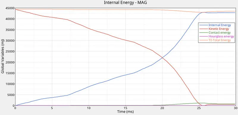
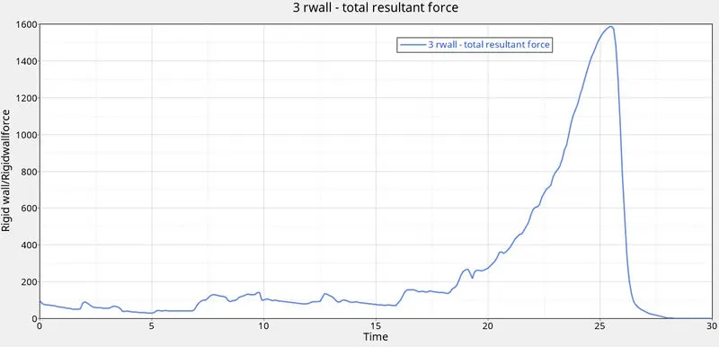
There is no slight difference between the graphs from previous cases. The deformation characteristics also similar from previous cases. we can conclude that there is no edge to edge penetrations in the crush tube.

Case 4:Remove both notches and remove boundary condition on rigid body node then run.

Import the 0000.rad file. NOw remove the notch in the model by selecting geometry>node edit>align node tool. select refernce nodes as 1st node and 2nd node. after that select the nodes that need to be align. now select align.

After the removal of notch, the model shown below.

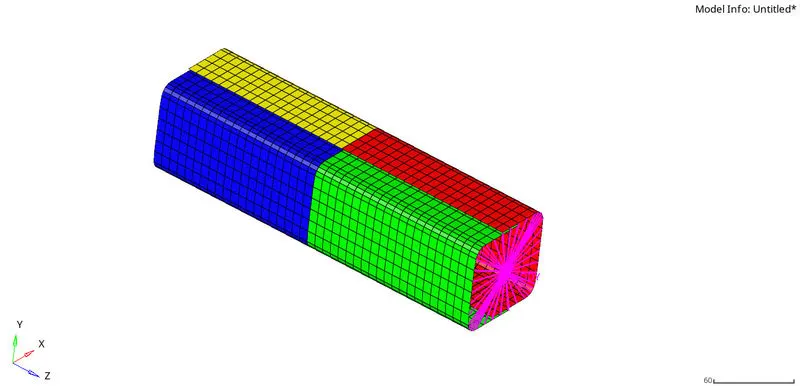
The next step is to remove the boundary conditions in solver browser,

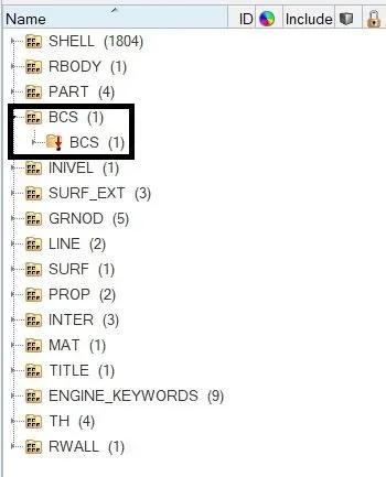
After that run the simulation by following the procedure of previous cases.

Now open the 0000.out file in file directory to check the energy errors, no.of.cycles and elapsed time in the simulation file.

As We can see the energy error is -1.4% and it is acceptable since it is below -15%. there is no mass error (0%).

Now run the animation by selecting hyperview in client selector. After that load the .h3d file.

To run the animation,the contour panel should be selected. after that select parameters such as result type as von mises, selection as components, averaging method as simple and then select apply to run the animation.

The animation shown below,

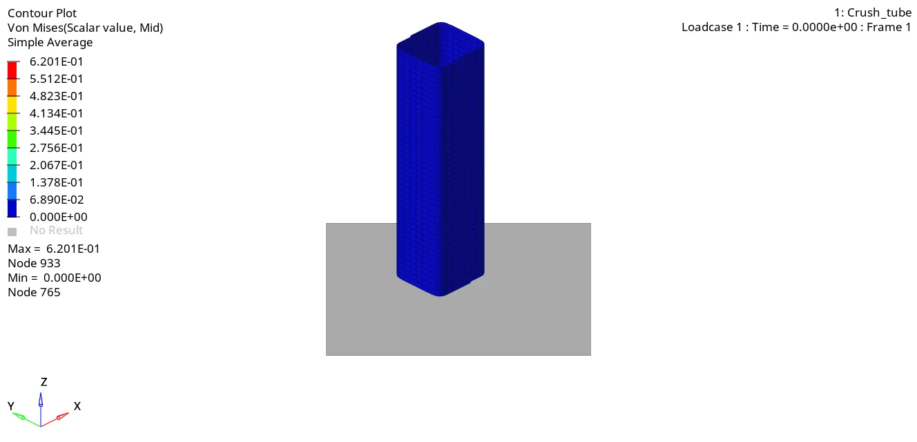
There is no notch present in the model, the buckling started at the contact takes place in rigid wall and tube. In previous cases, buckling started at notch areas.

Here we can switch to hypergraph 2D panel for plotting graph via client selector. In this panel, we need to load T01 file in file directory. Now select variable as Internal Energy, Kinetic Energy, total energy, contact energy, hourglass energy and select parameter as MAG and apply for plotting the graph.

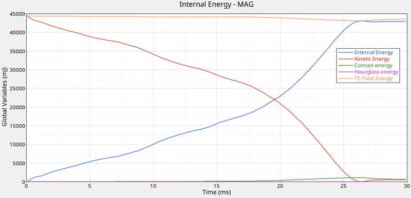
Internal energy keeps increasing at some point due to buckling of the tube. the more energy absorbed by the tube when deformation takes place. that's why the internal increases after some point.

Kinetic energy decreases from maximum due to internal energy increases.

Compared to previous cases, Contact energy slightly decreased after some point due to the absence of notch.

Total energy also slightly decreased after some point due to contact energy. Hourglass energy is constant due to the presence of recommended properties.

Next is to plot rigid wall resultant force graph for case 4 simulation, so select variable as rigid wall and parameter as resultant force and apply to plot the graph.

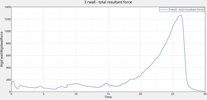
In this case, the RWALL force graph peaks after some point due to the large amount of force is transferred to the rigid wall during collision of the crush tube. After the deformation completed, the graph decreased suddenly. and got constant value after the deformation. The total resultant force peaks at 1200N.

Case 5:Create a new notch in the middle ,select the whole section and run.

In this case, we need to create notch in the middle. Import the 0000.rad file in case 4 directory by selecting import>solver deck. after that go to 2D>element offset tool to create the notch in the middle. select the elements need to offset and assign offset length as 3mm. Now select offset + to the selected elements offset downwards.

After the new notch is created in the middle as shown below,

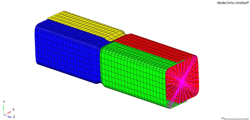
Now run the simulation by following the same procedure from previous cases.

Now open the 0000.out file in file directory to check the energy errors, no.of.cycles and elapsed time in the simulation file.

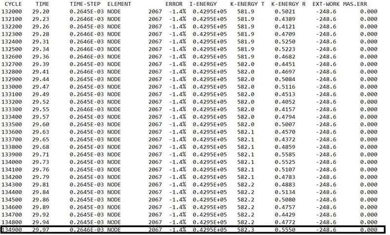
As We can see the energy error is -1.4% and it is acceptable since it is below -15%. there is no mass error (0%).

The next step is to run the animation by selecting hyperview in client selector. After that load the .h3d file.

To run the animation,the contour panel should be selected. after that select parameters such as result type as von mises, selection as components, averaging method as simple and then select apply to run the animation.

the animation shown below,

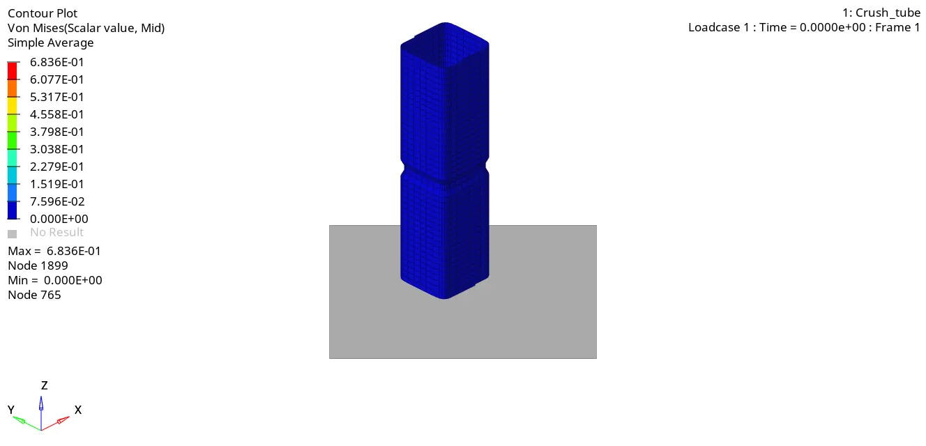
As similar in first 3 cases, the crush tube undergoes buckling at first where the notch is present. After that the lower part of the crush tube deforms next. After some milliseconds, the entire tube is crushed completely.

we need to switch to hypergraph 2D panel for plotting graph via client selector. In this panel, we need to load T01 file in file directory. Now select variable as Internal Energy, Kinetic Energy, total energy, contact energy, hourglass energy and select parameter as MAG and apply for plotting the graph.

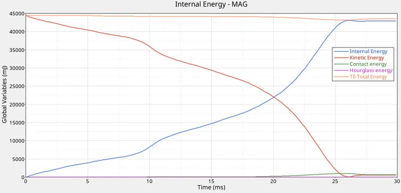
As we seen previous cases, Internal energy keeps increasing due to the deformation takes place. Kinetic energy also decreases due to increasing of internal energy. while contact energy slightly changed in earlyand also noticeable. it because the depth of the notch increased from previous cases. Total energy also increases earlier due to increasing of contact energy. Hourglass energy is constant due to the presence of recommended properties.

Next is to plot rigid wall resultant force graph for case 5 simulation, so select variable as rigid wall and parameter as resultant force and apply to plot the graph.

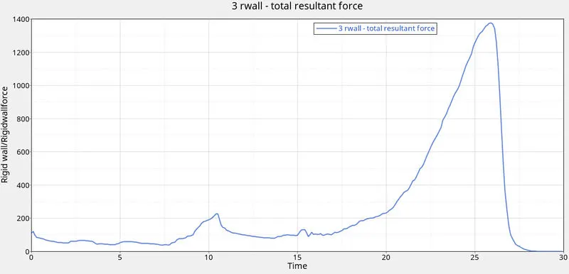
There is no noticeable difference between case 4 and case 5. its almost similar. after some point, RWALL force peaks at some value due to the absorption of energy created during collision. after the tube crushed completely, the value decreased and got constant.

Case 6:Create a new notch with nodes only from opposing 2 faces and run.

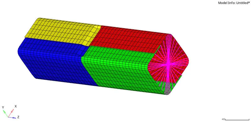
In this case, we need create a new notch with nodes only from opposing faces. Import the 0000.rad file in case 4 directory by selecting import>solver deck. after that go to 2D>element offset tool to create the notch in the opposing faces. select the elements from opposing faces need to offset and assign offset length as 3mm. Now select offset + to the selected elements offset downwards.

After the new notch is created in the middle as shown below,

After that run the simulation by following the procedure of previous cases.

Now open the 0000.out file in file directory to check the energy errors, no.of.cycles and elapsed time in the simulation file.

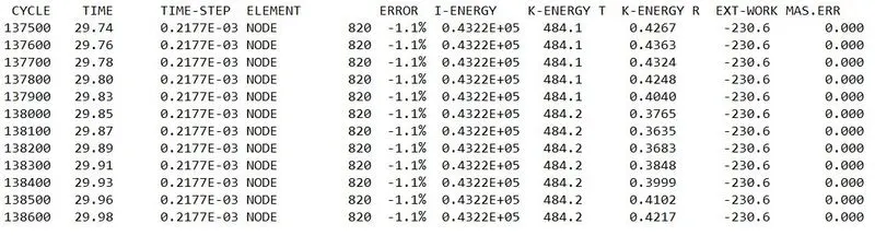
As We can see the energy error is -1.1% and it is acceptable since it is below -15%. there is no mass error (0%).

Now run the animation by selecting hyperview in client selector. After that load the .h3d file.

To run the animation,the contour panel should be selected. after that select parameters such as result type as von mises, selection as components, averaging method as simple and then select apply to run the animation.

The animation shown below,

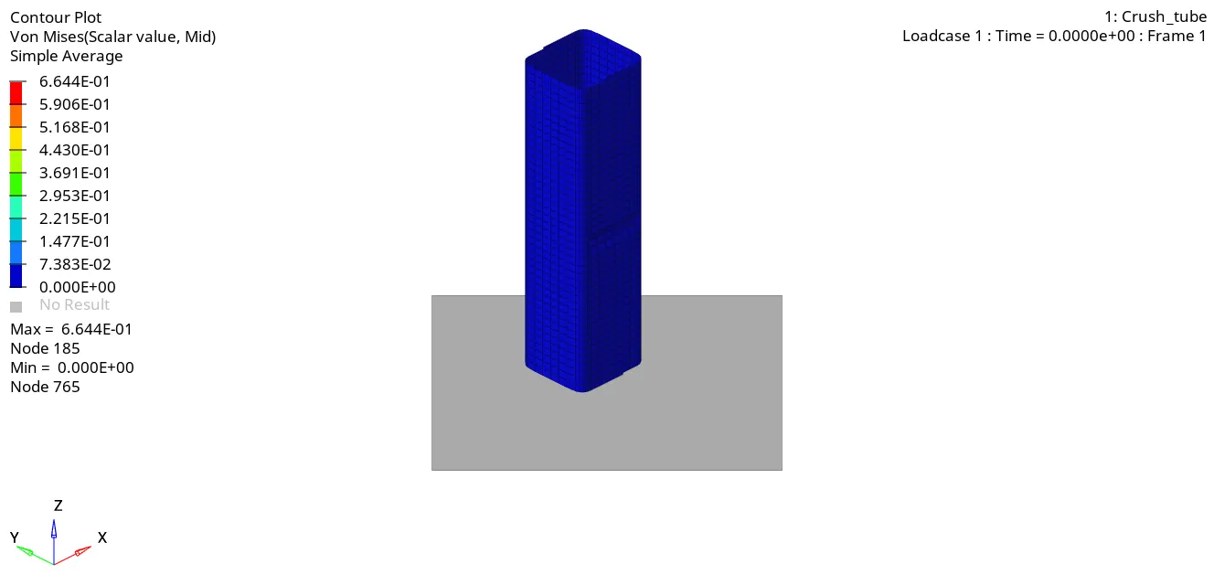
Like previous case, The buckling occurs at first the region where the notch is present. after that lower part of the tube deformed. finally the upper part deformed completely after some point.

Here we can switch to hypergraph 2D panel for plotting graph via client selector. In this panel, we need to load T01 file in file directory. Now select variable as Internal Energy, Kinetic Energy, total energy, contact energy, hourglass energy and select parameter as MAG and apply for plotting the graph and Next is to plot rigid wall resultant force graph for case 4 simulation, so select variable as rigid wall and parameter as resultant force and apply to plot the graph.

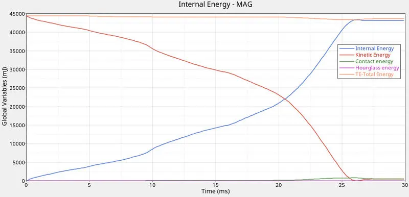
Like previous cases, the internal energy increases due to the deformation occurs. kinetic energy decreases from high value due to increasing of internal energy. The contact energy also noticeably increases due to the depth of the notch. Total energy increases due to contact energy increases after some point. Hourglass energy is constant due to the presence of recommended properties.

Next is to plot rigid wall resultant force graph for case 6 simulation, so select variable as rigid wall and parameter as resultant force and apply to plot the graph.

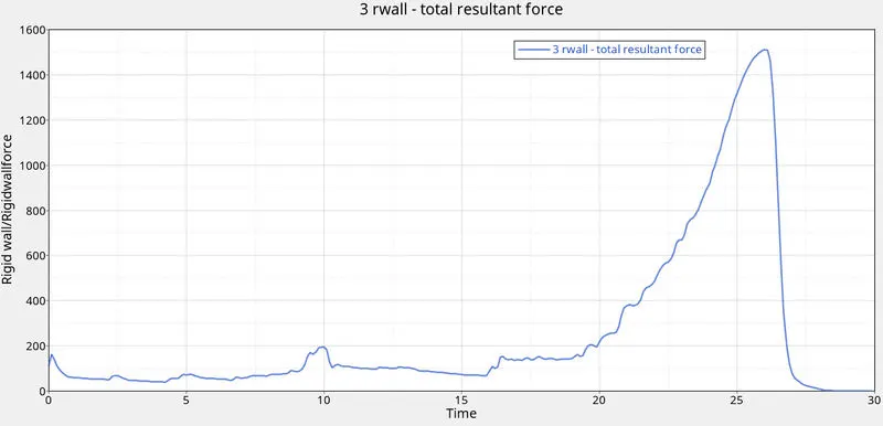
Again, the plotted RWALL graph is similar like previous case. In this case,the peak value is silghtly decreased due to the presence of notch only in opposing faces. After buckling process, the peak value drops to lesser and got constant after the tube crushed completely.

Results:

Comparison of results of all the cases:

Result for comparison	case 1	case 2	case 3	case 4	case 5	case 6
Energy error	-3.8%	-3.8%	-1.6%	-1.4%	-1.4%	-1.1%
Mass error	0	0	0	0	0	0
Internal energy	0.4202E+05	0.4202E+05	0.4287E+05	0.4297E+05	0.4295E+05	0.4322E+05
Kinetic energy	592.8	592.8	607.1	602.7	582.3	484.2
External work	-105.3	-105.3	-214.1	-201.0	-248.6	-230.6
Notches	present	present	present	no notches	Only at the middle	Only at the opposing faces

Final model of meshing:

Conclusion:

• The given bumper assembly is meshed with the mesh element size as 6mm.
• Done the simulation on a given crush tube model using various cases as mentioned above.
• plotted the energy graph and Rwall force graph for all cases and compared the final results.