Hyperelastic Material Models

Objective:

• calculate the different kinds of constants in hyperelastic material and compare both using stress-strain data from a Dogbone specimen tensile test with 100 percent strain.
• The given data is the engineering stress-strain in MPa/(mm/mm).
• The comparison should be shown from the d3hsp file and using simulation.

Theory:

Hyperelastic material model:

Rubber is generally considered to be fully incompressible since the bulk modulus greatly exceeds the shear modulus in magnitude. To model the rubber as an unconstrained material a hydrostatic work term, 𝑊𝐻(𝐽), is included in the strain energy functional which is a function of the relative volume, 𝐽,

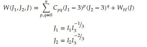
Mooney-Rivlin model has constant values. here we need to give an input curve using given data. Define the material model and define N value as 1, load the data as a curve in the material card. Now define required keywords. run the simulation. Quit the simulation after the simulation was started. Now open the d3hsp file. Now extract the constant values C01, C10 for N=1 in the model. Now open the same model. here we need to change the N value as 0 in the material card. Now define the constant values that we already got from the d3hsp file for N=1. Now run the simulation. Get the output results. We need to do a similar procedure for N=2, N=3 in the material card.

Procedure:

Now use the given engineering stress and strain values in the image for load curve input in the Material card.

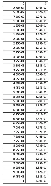
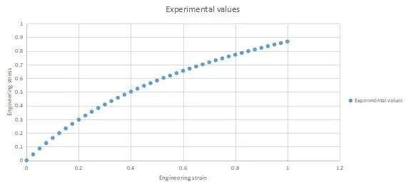
At first, Open the keyword file using open>ls-dyna keyword. Now the dogbone specimen model is imported.

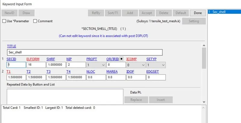
Now define the section id for the model. Go to model&keywords>all>Section>shell. define sec id, elform-16 for full integration points, thickness-1.5mm. Now accept and done.

Define the curve for the material card. Go to model&keywords>all>define>curve. Here we need to load the data points in the given image. select load xy tab and select the extracted data points. now apply and done.

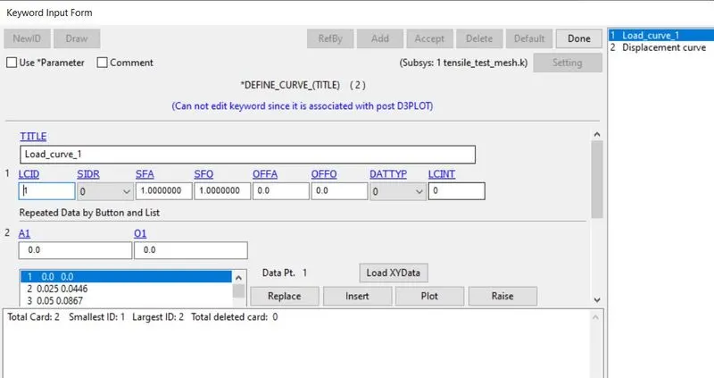
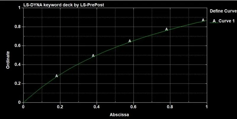
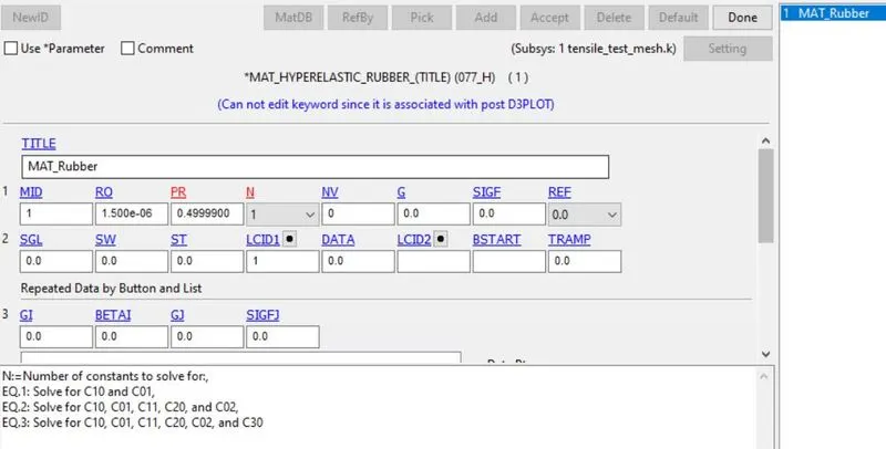
Now define the material card. Go to model&keywords>all>MAT>MAT_77(hyperelastic_rubber). Now define mat id, young's modulus, Poisson's ratio as 0.49 because Poisson's ratio should be greater or equal to 0.49. Now select N as 1. define curve id as 1.

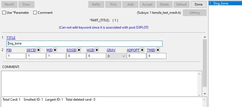
Define the part id, Go to model&keywords>all>part. Now define the sec id, mat id. Accept and done.

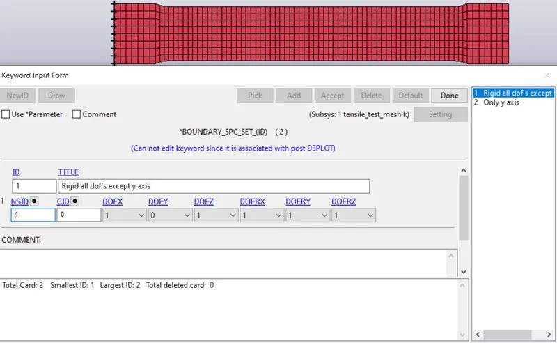
Define boundary conditions using model&keywords>all>boundary>spc. Constraint all DOF's except Y-axis.

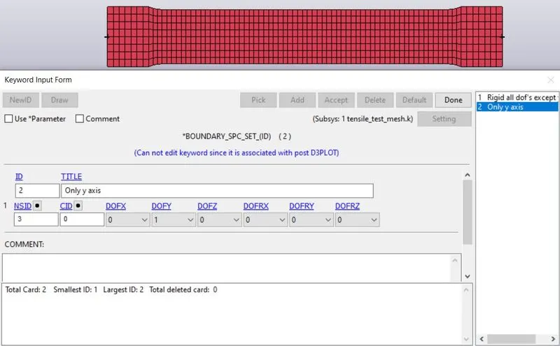
Define boundary conditions using model&keywords>all>boundary>spc. Constraint only Y-axis.

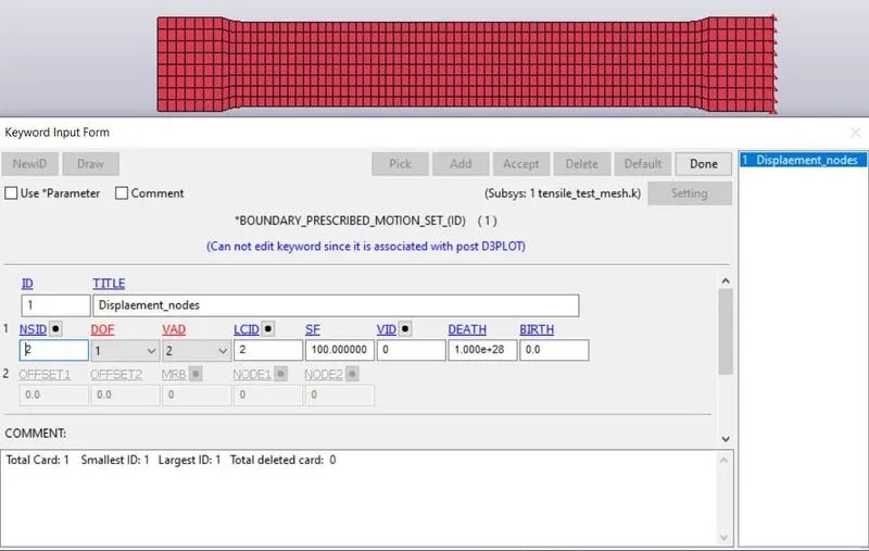
Define boundary conditions using model&keywords>all>boundary>Prescribed_motion_set. Assign DOF as 1(x-axis), VAD as 2(for displacement), LCID as 2.

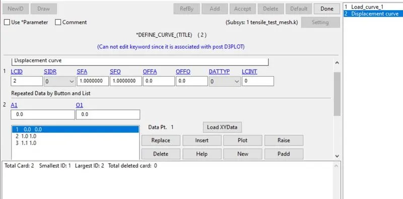
Define curve for the displacement for the model. Go to model&keywords>all>define>curve. Now insert the values for the displacement and select accept&done.

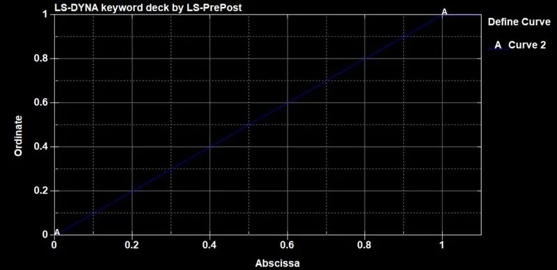
Defining Control card:

Define control termination card for the simulation. Go to Go to model&keywords>all>Control>termination. Define DT as 0.01.

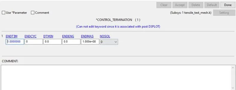
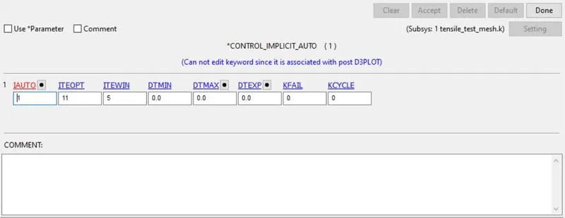
Control cards for implicit analysis:

implicit_auto:

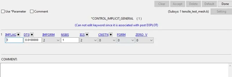
implicit_general:

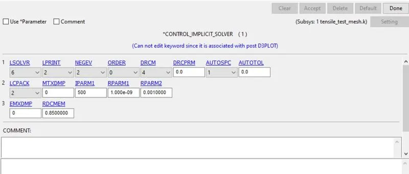
implicit_solver:

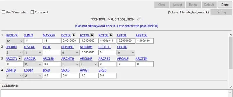
implicit_solution:

Defining Database:

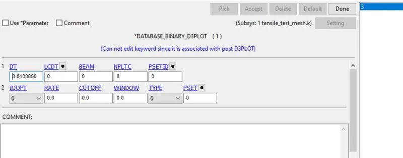
Define binary d3plot output requests using model&keywords>all>database>binary d3plot. Define DT as 0.01.

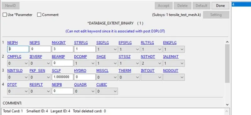
Define Extent_binary using model&keywords>all>database>Extent_binary. define STRFLAG as 1.

Define ASCII using model&keywords>all>database>ASCII. define GLSAT, MATSUM as 0.01.

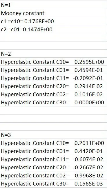
Now run the simulation. Get the Mooney-Rivlin constants values using the d3hsp file. the constant values are shown below for N=1, 2, 3.

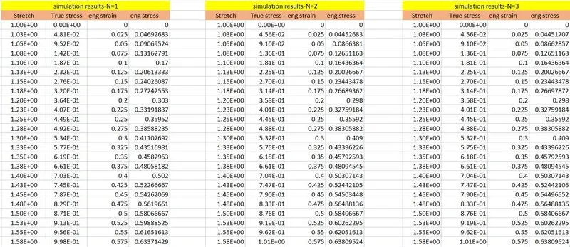
Now the extension and true stress values are extracted from the d3hsp file for N=1,2,3.

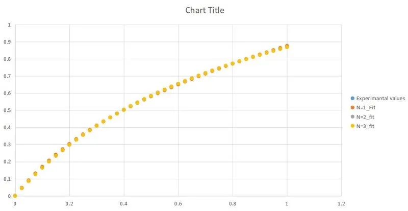
Validation of the Material card using constant values in N value:

Now define the N value as 0 and Assign constant values from the d3hsp file from N=1,2,3 modes instead of the loading curve for all the N=1,2,3.

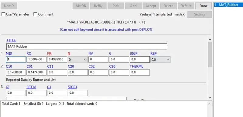
After run the simulation. Now plot the X-stress and X-strain values versus time using d3plot file.

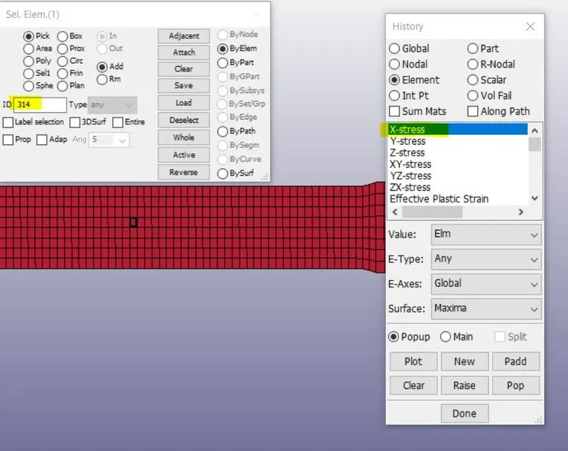
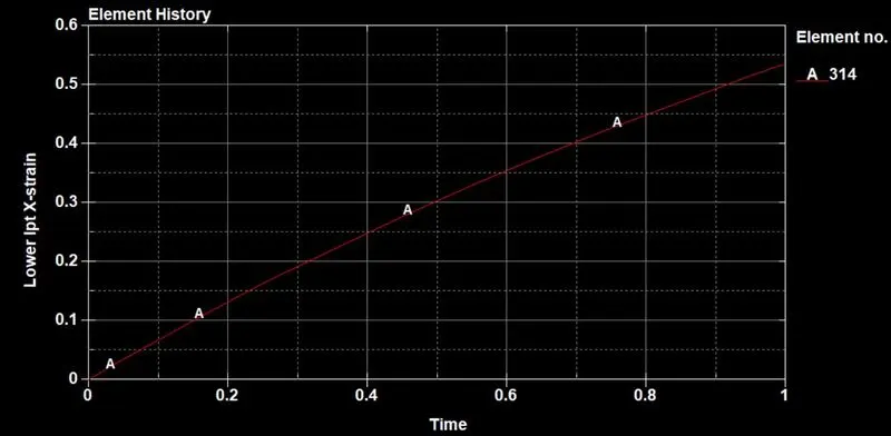
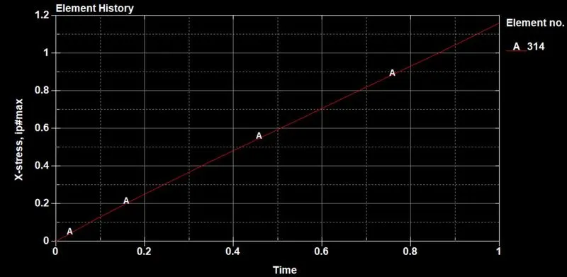
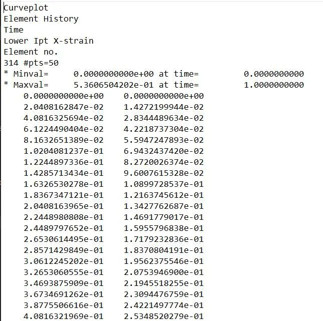
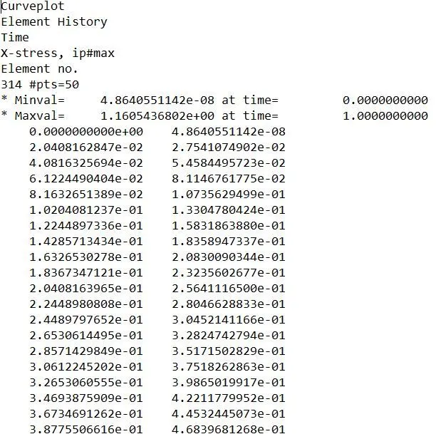
Now plot the stress vs strain using cross plot of stres-strain vs time graph.

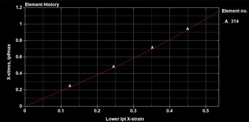
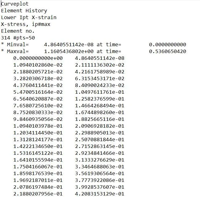
Now we got true stress vs true strain values. we need to convert to engineering stress vs strain values to compare the results from experimental and simulation values.

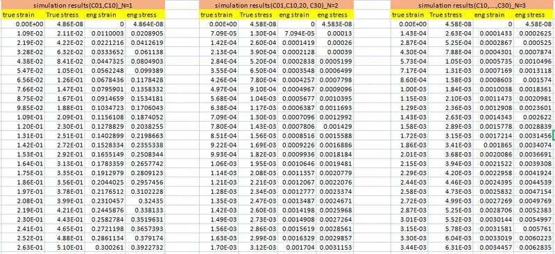
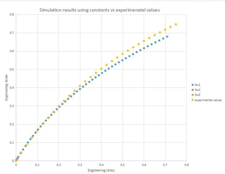
Now compare the experimental and simulation result values of engineering stress vs engineering strain values.

Conclusion:

• The Mooney-rivlin constant values are obtained from the d3hsp file when run the simulation using polynomial N=1 and load the given engineering stress and strain values.
• Converted the Stretch vs stress values from d3hsp file. compared with experimental values and found it to be close fit.
• Defined the mooney-rivlin constant values in the material card and again ran the simulation. Got the stress-strain plots using d3plot file.
• Compared the experimental values with simulation result values.