Assignment 4-RADIOSS Material Laws Challenge

Objective:

1. To do simulations of the starter file using various cases as mentioned in the question above.

2. To plot graphs for the obtained values from those cases.

3. To compare the results from those cases and conclude why the failure happened.

Theory:

In general, The material plays the prominent role in simulations. The accuracy of the simulation depends on material chosen. Choosing the right material and providing the right material data in performing a simulation is very important.

In radioss, The materials are categorized into two ways. There are based on material cards (using laws) and based on material properties.

Based on material cards (using laws):

• Law 1- represent the linear elastic materials (isotropic elastic material).
• Law 2- represent the johnson-cook material (isotropic elasto-plasto material).
• Law 27- represent the elastic-plastic brittle material (isotropic elasto-plasto material).
• Law 36- represent the elastic- plastic piecewise material (isotropic elasto-plasto material).
• Law 42- represent the odgen (rubber like) material (viscous material)
• Law 70- represent the foam material (viscous material)

Based on material property:

• isotropic elastic
• isotropic elasto-plastic
• composite & anisotropic materials
• viscous material
• hydro-dynamic material
• explosives.

Isotropic elastic material (using Law 1):

Isotropic means that a material will have the same material properties in all three directions. Elastic means that the material has the ability to retain back its original shape after removing the stress. In radioss, Law 1 is exclusively for elastic material. This law follows hooke's law of elasticity. It is available for trusses, beams, shell and solid elements. The material stiffness is determined by young's modulus and poisson's ratio. This law is used for small deformation.

Isotropic elasto-plastic material (law 2 & law 36 & law 27):

Law 2_Johnson cook material:

This law represent that a material which possess both elastic and plastic property along with isotropic properties.Model expresses material stress as a function of strain, strain rate and temperature. when plotting the graph, it starts from yield stress point where as `sigma`-stress, `epsilon`p- plastic strain,a-yield stress, b-hardening modulus(how well the curve bends), n-hardening exponent(how quick the curve bends from vertical to horizontal direction), c- strain rate coefficient,`epsilon`-strain rate, `epsilon`0-reference strain rate.

If the material is not temperature or strain rate sensitive, then the temperature ans strain rate is neglected.so we can calculate a, b, n values. 

In material card, we have a option called eps_max which known as plastic strain at failure. Failure of the element happens when the integration point 1 reaches eps_max. Now if the failure is only based on eps_max. there can be instances where tha eps_max gives out unrealistic results. To avoid this we have the option failure johnson cook card.

Johnson hook failure model:

This card provides the user to more control over the failure of the johnson hook strain.Here we can use d1,d2,d3 values and SIG_y, UTS, EPS_UTS  values to calculate a, b, n values. We use ixfem values fro element deletion. ixfem=0 for simply deleting the element, ixfem=1 for break the elements as per the force and load conditions. ixfem is only used for shell elements.

Law 36_elasto-plastic piecewise linear material:

This law is represented by PLAS_TAB. It has some advantage that the lab data which is real it given to the software in the form of stress-strain curve. it allows us to import the user defines functions. This law is the widely most used material model in industrial.it can be used for all shell and solid elements. it had an advantage to add johnson cook failure model as well.

the law 36 model has 4 damage and rupture parameters,

• EPS_MAX- maximum plastic strain for element deletion for any loading like tensile, compression or shear.
• EPS_t- the begining of the tensile damage.
• EPS_m- the end of the tensile damage. the stress is null but the element is not deleted.
• EPS_f- tensile failure strain value for element deletion.
• EPS_1- large principal strain.

Law_27 elasto plastic material law for brittle failure:

This law has isotropic elasto-plastic johnson-cook material with orthotropic brittle failure model. This law is specially used for brittle materials like aluminium and glass. Material damage and failure happens only in tension.This material law is applicable for shell elements. Same as law 36, it has damage and rupture parameters like EPS_t,EPS_m,EPS_f, Dmax where Dmax is the damage factor (which accelerates the failure of element).

Viscous model(law 42 & law 70):

Law 42-odgen material:

Hyper elastic behaviour that is non linear elastic. Generally used to model plolymers and rubbers. it has multiple inputs to pertaing bulk modulus. also has prony series parameters.

Law 70- tabulated foam materials:

It is used for the application with foam material. It has an advantage that absorbs energy without developing the stress.

Procedure:

Case 1- Run base simulation without any changes:

At first, import the solver deck and import the model which end at _0000.rad file. Select radioss as solver deck.

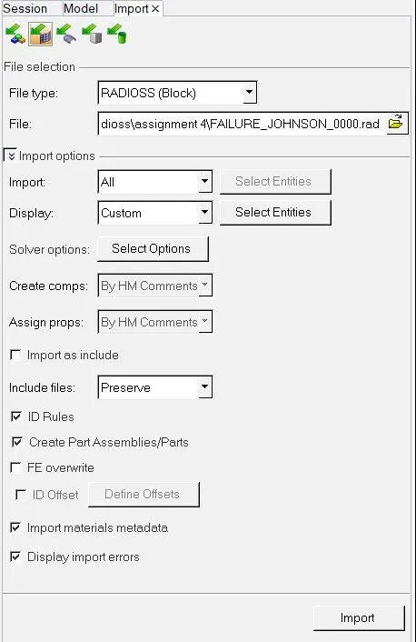
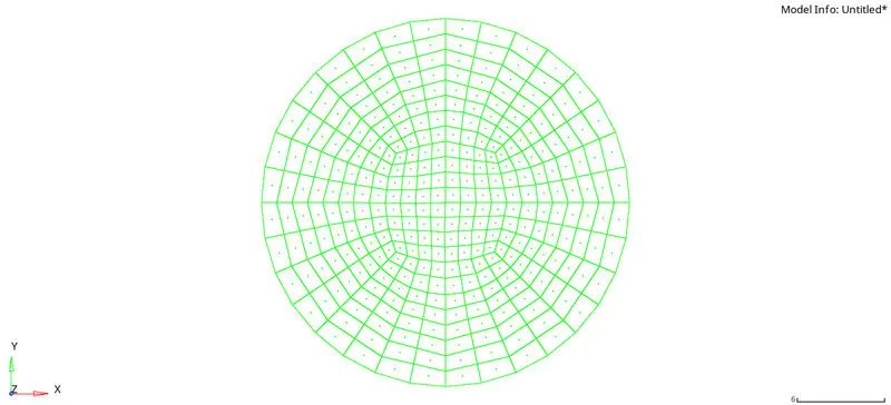
after importing the file, the model is in wireframe mode, so we need to change the mode to shaded element with mesh lines. The model appears as shown below.

 

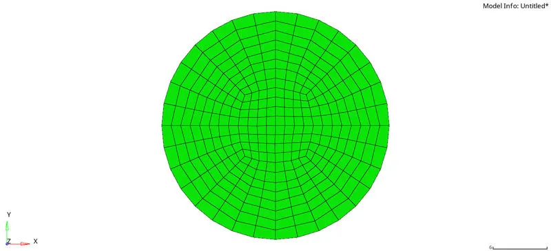
Now in solver browser, we need to check some card for verifying to clarify some aspects. the first card 'begin card' to be checked for unit system. the unit system plays important role in assigning values.

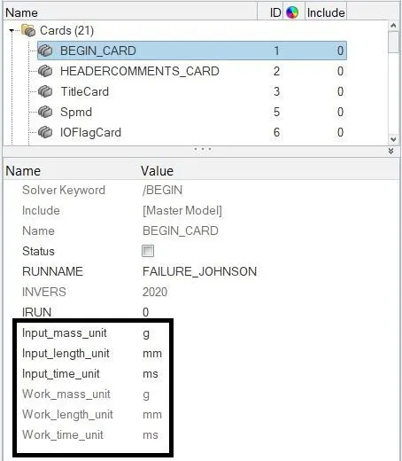
Now check the material card that the values are assigned properly and verified it.

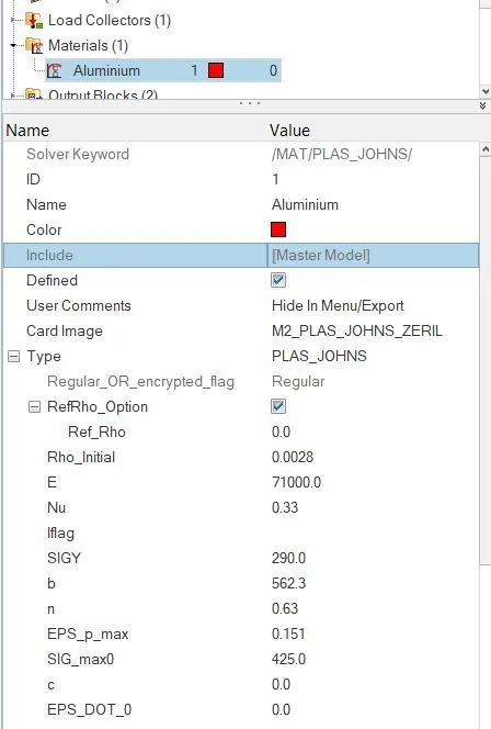
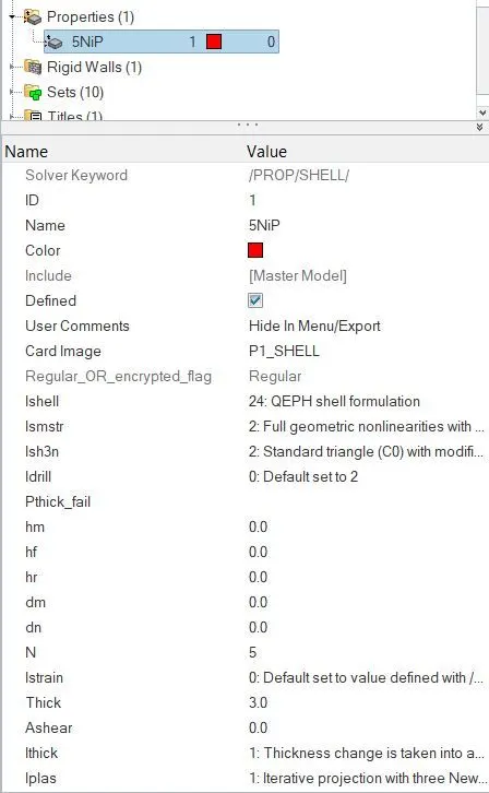
select property card and verify the recommended shell properties are assigned correctly.

Here in this case we need to run base simulation without any change. so got to analysis>radioss. select save as to select the path for saving the simulation files. In option tab, type -nt 4 for increasing the speed of the cores to run the simulation fastly. then click radioss.

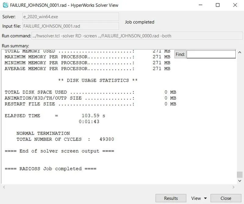
It take a few minutes, after the completion of simulation,  the window pops up to shown the history of the simulation files.

Now go to file directory where the files are saved, open 0001.out file in notepad for seeing energy error, mass error, internal energy, kinetic energy etc.,

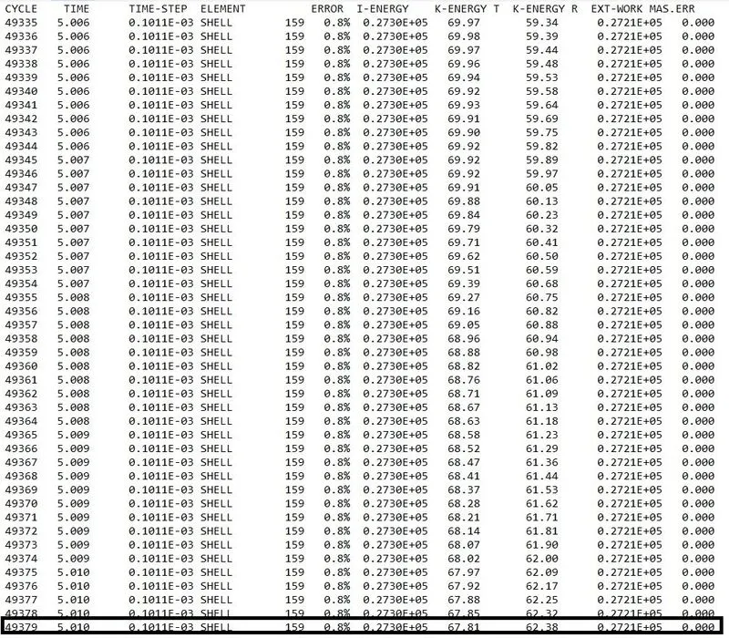
The obtained last cycle values are 

energy error=0.8%

kinetic energy=67.81 KJ

internal energy=0.2730E+05 KJ

mass error=0

total no.of.cycles=49380

Elapsed time=139.41 s

The next step is to view simuation by selecting hyperview in client selector. After open the hyperview, load the h3d file in file directory. 

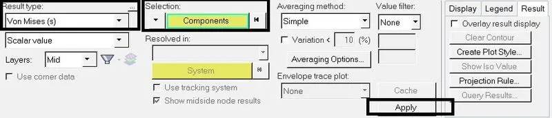
To run the animation,the contour panel should be selected. after that select parameters suc as result type as von mises, selection as components, averaging method as simple and then select apply to run the animation.

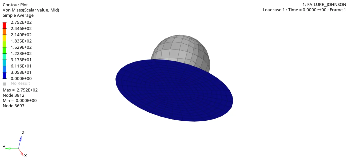
The simulation is shown below, 

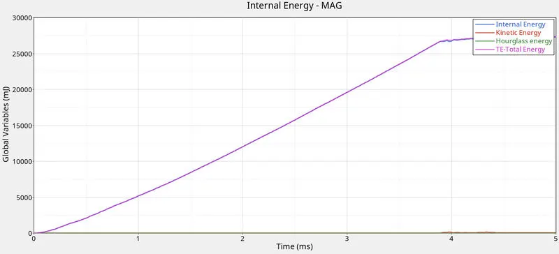
The next step is to plot the graphs for resultant rigid wall forces, internal energy, kinetic energy, toatl energy, hourglass energy. Here we can switch to hypergraph 2D panel for plotting graph via client selector. IN this panel, we need to load T01 file in file directory. NOw select variable as I.E, K.E, total energy and select parameter as MAG and apply for plotting the graph.

In this energies graph, the internal energy increases gradually from origin due to gradual increase in displacement.

The total energy is the combination of all energies, so the graph increases gradually from origin.

The hourglass energy is constant because we used recommended shell properties to avoid hourglass effect.

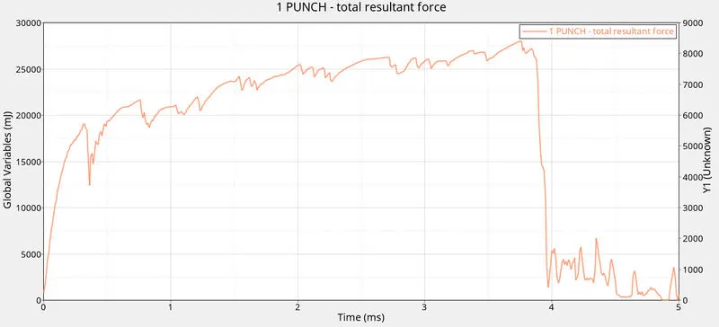
Now next step to plot rigid wall resultant force graph for base simulation, so select variable as rigid wall and parameter as resultant force and apply to plot the graph.

The obtained graph explains us , the sphere shaped model absorbs energy initially, and once the rigid ball hits the plate the graph reaches the peak values due to energy absorbtion. after reaching the rupture point, the element got deleted and the values down to zero.

Case 2- changing the values in failure card:

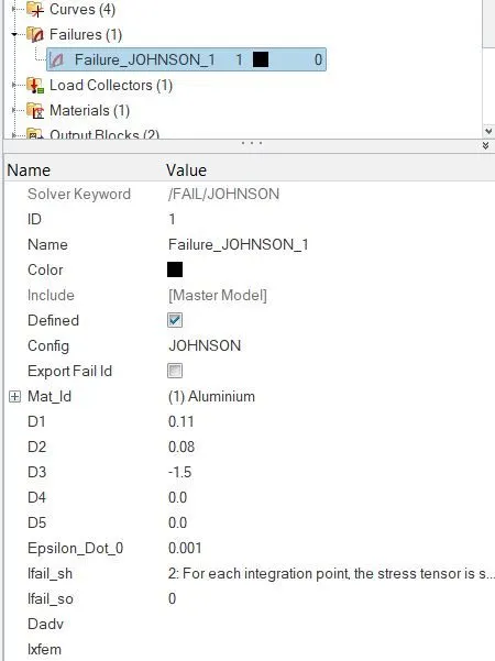
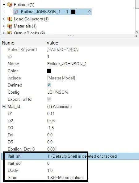
In this case, the failure card will have some changes. we should change some values in this card. te material card is Law 2 as same as case 1. In failure card, we need to change the values as Ifail_sh=1, Dadv=1, Ixfem=1.

 

Now go to analysis>radioss, run the simulation as follow the same procedure above. after selecting the radioss it takes few minutes to run the results and the results window pops up.After that, the next step is to open 0001.out file to check the energy error, mass error, internal energy, kinetic energy etc.,

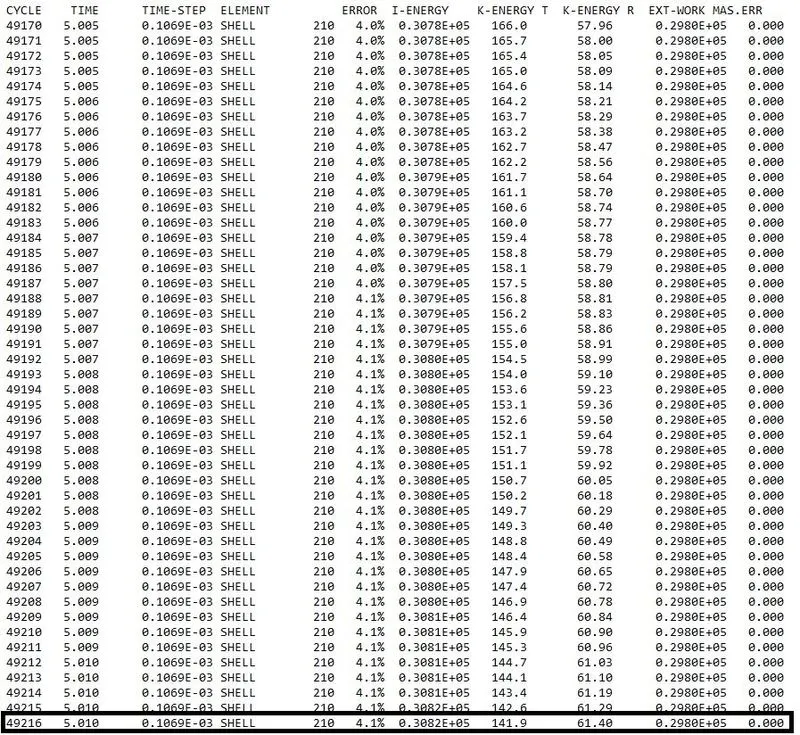
The obtained last cycle values are 

energy error=4.1%

kinetic energy=141.9 KJ

internal energy=0.3082E+05 KJ

mass error=0

total no.of.cycles=49217

Elapsed time=149.43 s

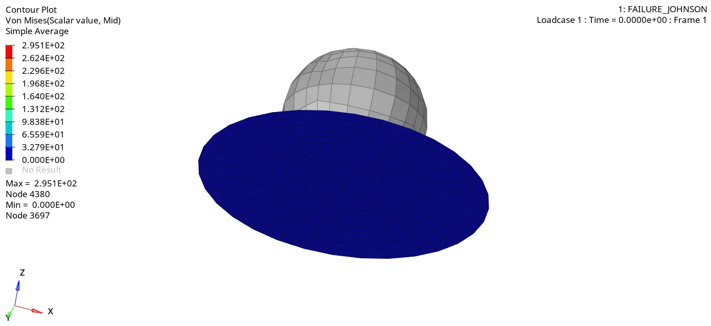
the next step is to switch the panel to hyperview. Load the h3d file. Now assign the given parameters as von mises, simple and then apply to run the animation.

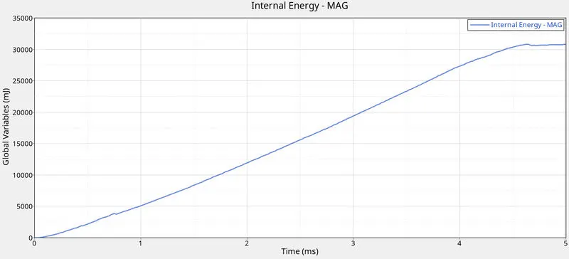
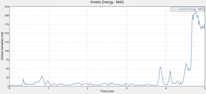
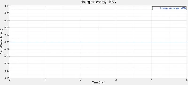
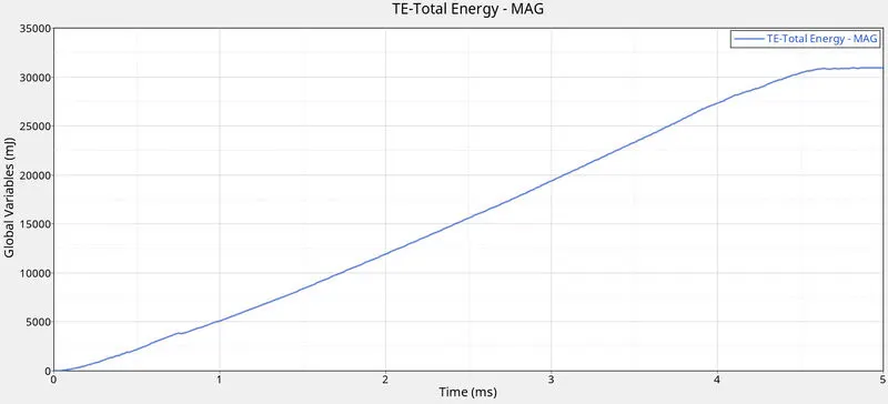
The next is to plot the energy graphs by switching to hypergraph 2D panel, Now load the T01 file and select the variables as  internal energy, kinetic energy, hourglass energy, total energy and select apply to plot the graphs.

The internal energy increases gradually from the origin and reaches the peak value and due to element breakage, the value decreases bit low.

the kinetic energy varies from origin after the breakage of elements the values are raised at peak and decreased suddenly.

Due to assigning the recommended shell properties, the hourglass energy is constant.

the total energy is the sum of all energies. it increases due to increase of kinetic and internal energy.

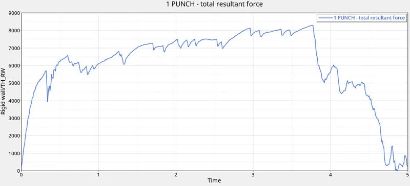
Now the plot resultant rigid wall force graph by changing the variables as rigid wall. and the obtained graph is reaches peak value after the element reaches rupture point the values gets down to zero.

Case 3- Deleting the failure card:

In this case, we need to delete the failure card in the 0000.rad file in solver browser.

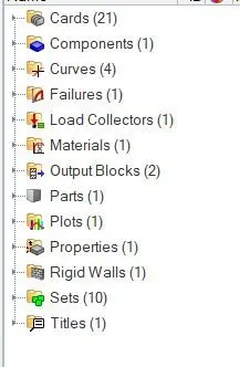
After deleting the card, the remaining cards are shown below.

Now follow the procedure in case 2 to run the simulation without any further changes in the cards.

Now open 0001.out file in path directory to check the energy error, mass error, internal energy, kinetic energy etc.,

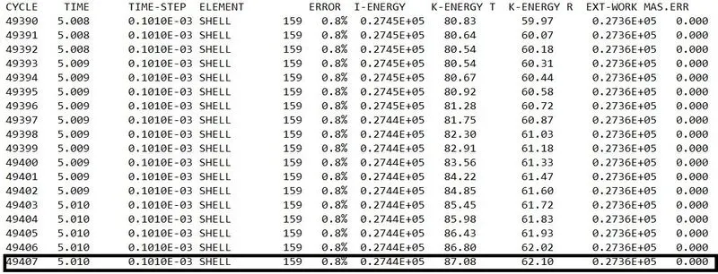
The obtained last cycle values are 

energy error=0.8%

kinetic energy=87.08 KJ

internal energy=0.2744E+05 KJ

mass error=0

total no.of.cycles=49408

Elapsed time=139.29 s

Now switch the panel to hyperview. Load the h3d file. assign the  parameters result type as von mises, selection as components, averaging method as simple and then apply to run the animation.

The animation shown below,

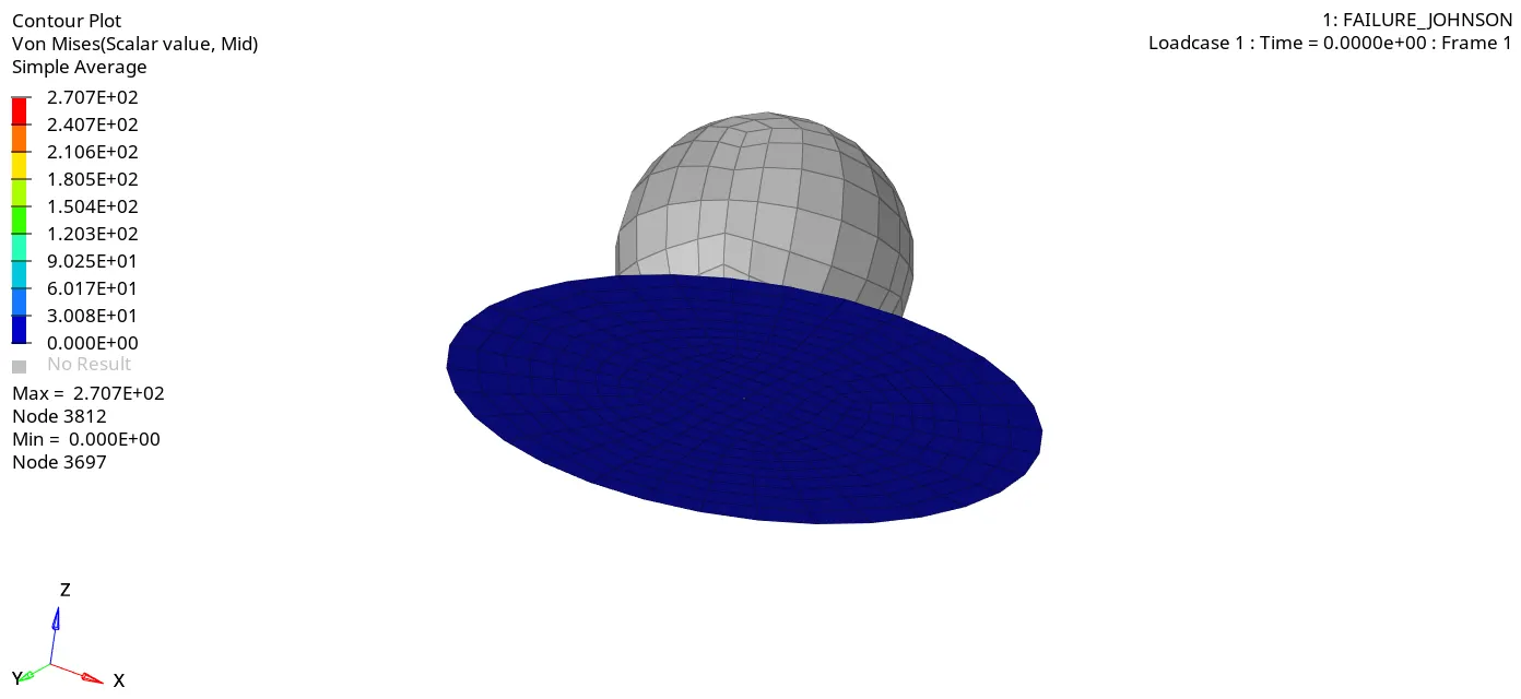
Now plot the energy graphs by switching the panel to hypergraph 2D panel, Now load the T01 file and select the variables as internal energy, kinetic energy, hourglass energy, total energy and select apply to plot the graphs.

The internal energy graph is plotted, it is similar to the previous case.

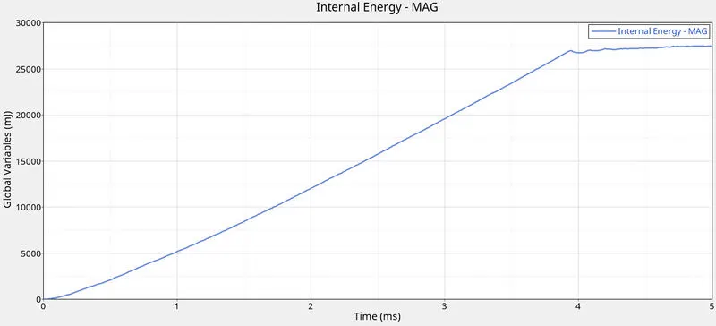
The kinetic energy graph is plotted, it is constant when the rupture point reaches the graph reaches peak value and get down to zero suddenly due to element deletion.

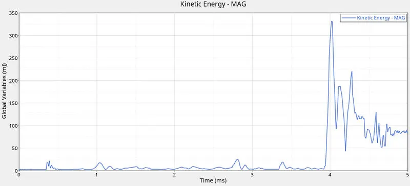
the hourglass energy is constant due to assigned the recommended shell properties.

the total energy  increases due to increase of I.E and K.E.

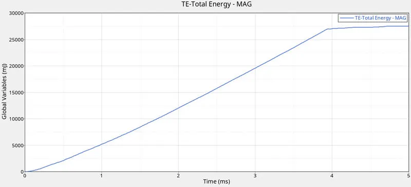
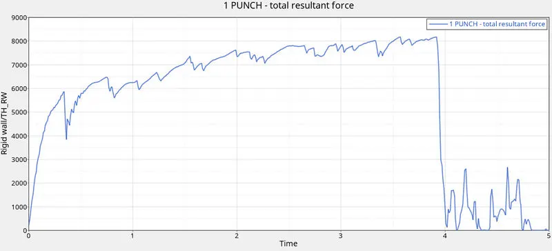
Now plot the resultant rigid wall forces graph by changing the variable as rigid wall and resultant force.

The obtained rigid wall force graph,

Case 4-Deleting the EPS_max value from the material card:

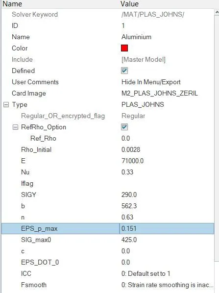
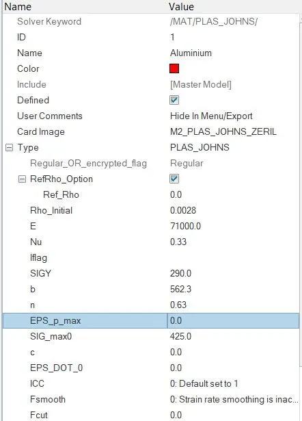
In this case, assign the EPS_max (plastic strain) value as 0 instead of 0.151. the changed card image as shown below,

 

Now run the simulation by follow the previous case procedure.

After the simulation is done. open 0001.out file in path directory to check the energy error, mass error, internal energy, kinetic energy etc.,

The obtained last cycle values are 

energy error=3.0%

kinetic energy=2.969 KJ

internal energy=0.6487E+05 KJ

mass error=0

total no.of.cycles=48737

Elapsed time=133.32 s

the next step is to switch the panel to hyperview. Load the h3d file. assign the  parameters result type as von mises, selection as components, averaging method as simple and then apply to run the animation.

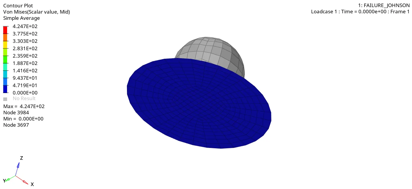
The animation shown below, the element will not break due to the value of EPS_Max as zero. so the element will not get deleted.

the next step is to plot the energy graphs by switching the panel to hypergraph 2D panel, Now load the T01 file.

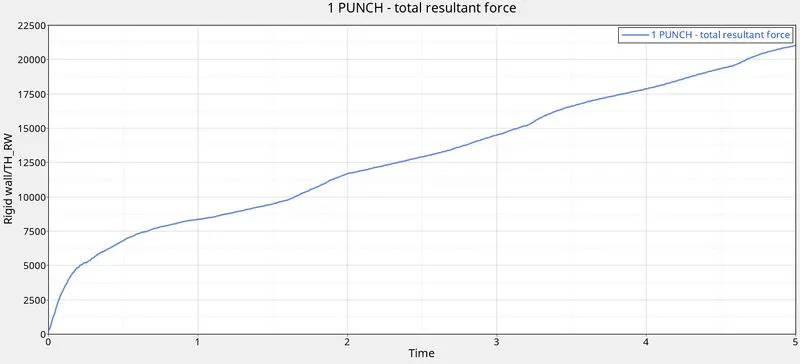
Plot the rigid wall force graph by selecting variables as rigid wall and resultant force and then apply. the graph is plotted. the graph shows us the value reaches peak due to the collision over the elements and the element reaches point of rupture. it get down.

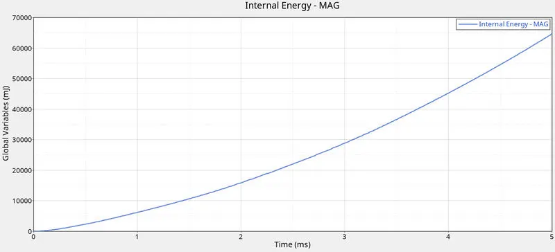
Now select the variables as internal energy, kinetic energy, hourglass energy, total energy and select apply to plot the graphs.

Internal energy is plotted, its increases gradually from the origin.

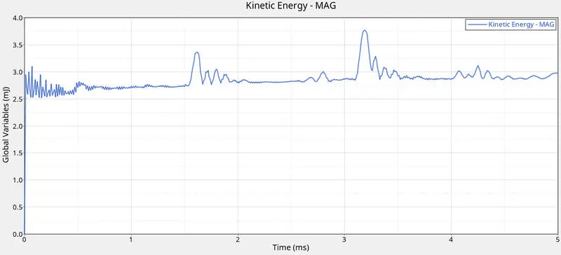
kinetic energy is plotted, it is constant when the ball get collide the energy reaches peak value and after collision the graph decreases.

hourglass energy is constant due to the present of recommended properties.

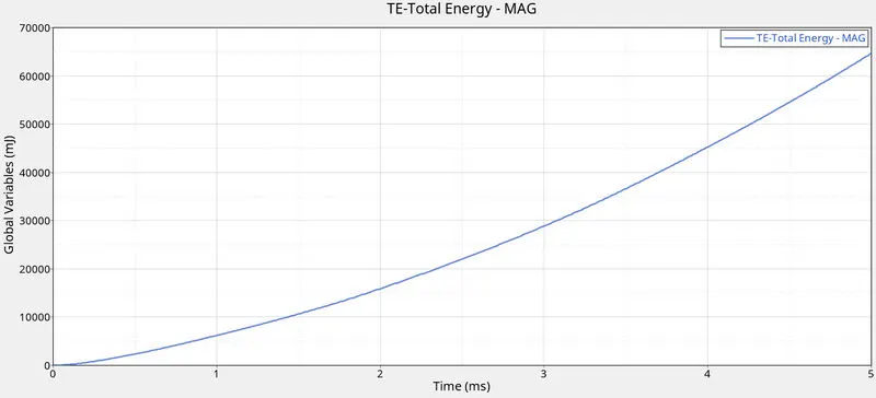
the total energy increases due to increasing of kinetic and internal energy.

Case 5-changing the material card to Law 1(linear elastic):

In this case, we need to change the material card to law 1 from law 2 as shown below, law 1 possess only elastic behaviour.

 

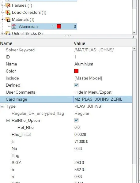
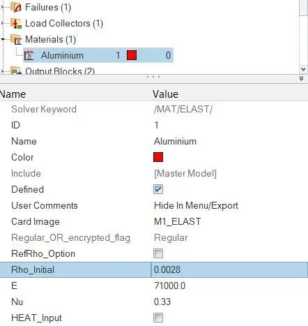
Now run the simulation by follow the previous case procedure.

After the simulation is done. open 0001.out file in path directory to check the energy error, mass error, internal energy, kinetic energy etc.,

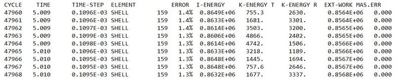
The obtained last cycle values are 

energy error=1.3%

kinetic energy=1677 KJ

internal energy=0.8632E+06 KJ

mass error=0

total no.of.cycles=47969

Elapsed time=126.37 s

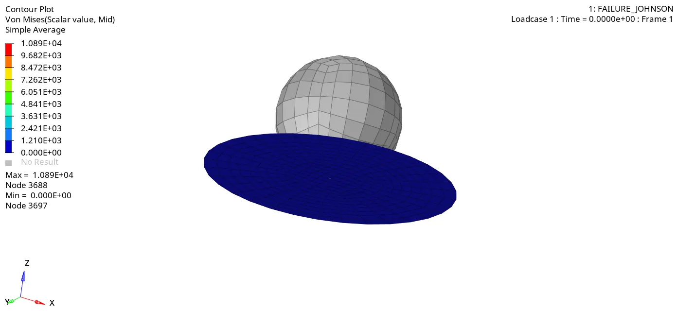
the next step is to switch the panel to hyperview. Load the h3d file. Now assign the given parameters as von mises, simple and then apply to run the animation. Here the element will not break due to the present of law 1. Law 1 represent only the elastic behaviour. so the model reaches till the yield stress point.

Now plot the energy graphs by switching the panel to hypergraph 2D panel, Now load the T01 file and select the variables as internal energy, kinetic energy, hourglass energy, total energy and select apply to plot the graphs.

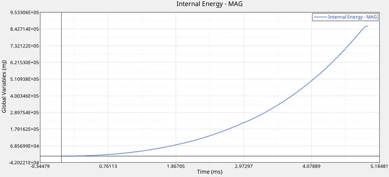
Internal energy is plotted, it increases gradually and get constant some point due to law 1 card, the material reaches only yield strength point.

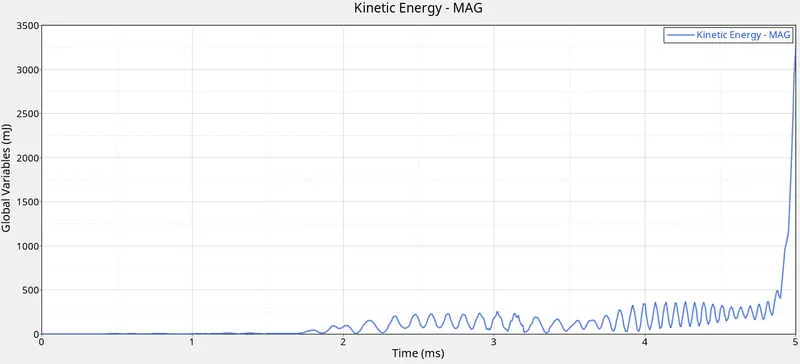
kinetic energy is plotted, it is constant when the ball get collide the energy reaches peak value.

Hourglass energy is constant due to the present of recommended properties.

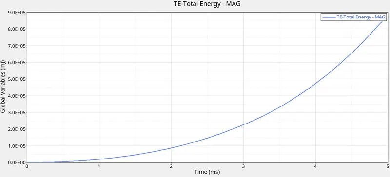
total energy is similar to the internal energy as shown below.

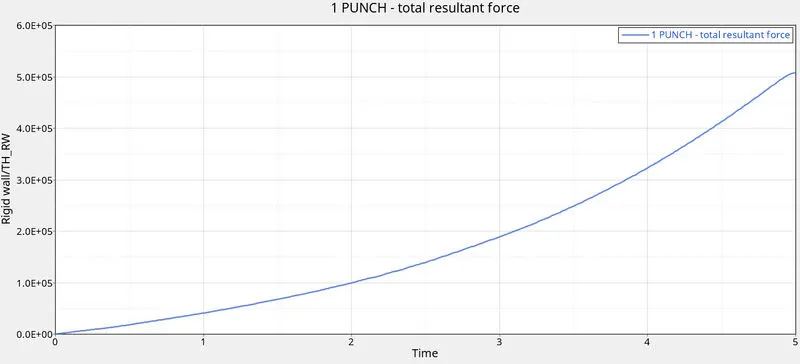
Plot the rigid wall force graph by selecting variables as rigid wall and resultant force and then apply. the graph is plotted. the graph increases gradually till the end. it doesn't decreases because there is no plastic behaviour takes place.

Case 6- Changing the material card to law 36 and assign parameters as given above:

In this case, we need to change the material card to law 36 (elasto plastic piecewise material) and assign values for parameters in material card as given above. change shell properties to recommended properties.

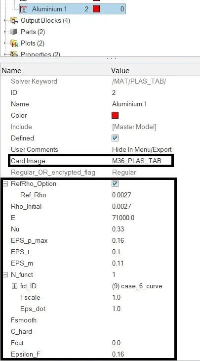
When defining the material card as law 36, a function should be represented to define the curves. At first some curves are defined. we need to define new curve as a function. the values are given by the user in question. by selecting create>curve>new>assign name>proceed.

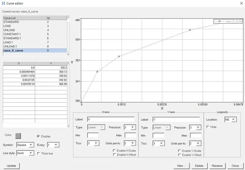
Now put the user given values in the x and y tab and select update to plot the curve. Now assign function>curve>case 6 curve.

After assigned the values, run the simulation.

Now open 0001.out file in path directory to check the energy error, mass error, internal energy, kinetic energy etc.,

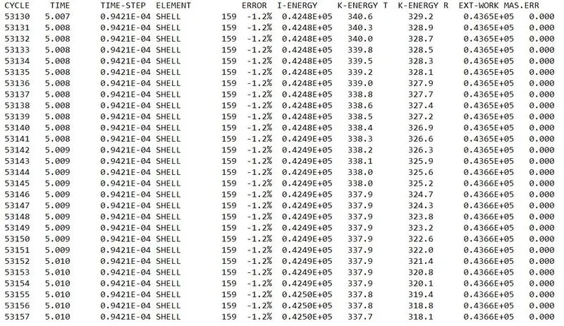
The obtained last cycle values are 

energy error=-1.2%

kinetic energy=337.7 KJ

internal energy=0.4250E+05 KJ

mass error=0

total no.of.cycles=53159

Elapsed time=140.53 s

the next step is to switch the panel to hyperview. Load the h3d file. assign the  parameters result type as von mises, selection as components, averaging method as simple and then apply to run the animation. the animation shown below,

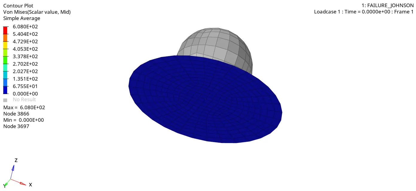
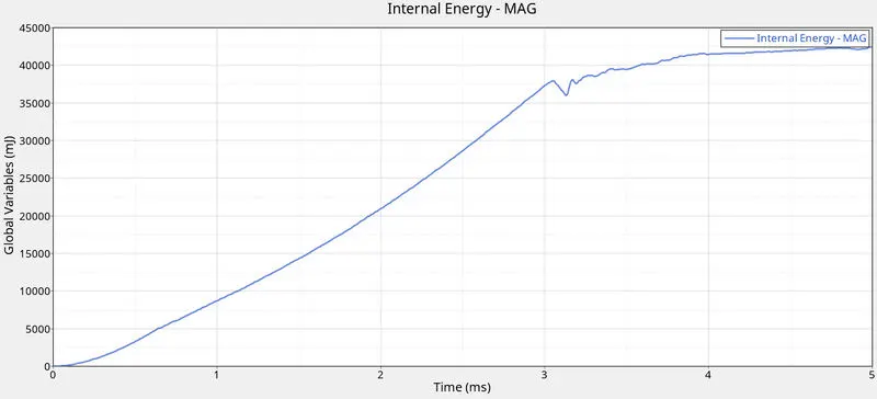
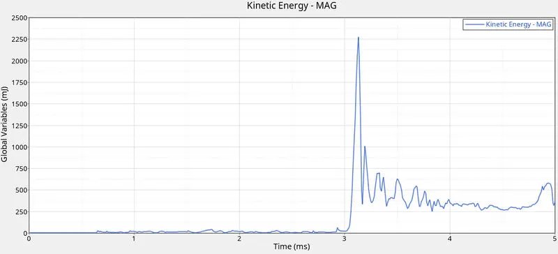
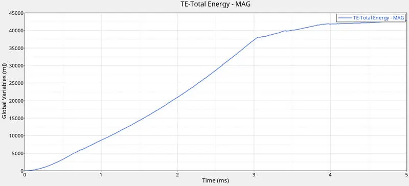
Now plot the energy graphs by switching the panel to hypergraph 2D panel, Now load the T01 file and select the variables as internal energy, kinetic energy, hourglass energy, total energy and select apply to plot the graphs.

The internal energy is plotted shown below, the graph increases gradually till the end.

The obtained kinetic energy is plotted below,

Hourglass energy is constant due to the presence of recommended shell porperties.

total energy is similar to internal energy. it is plotted below,

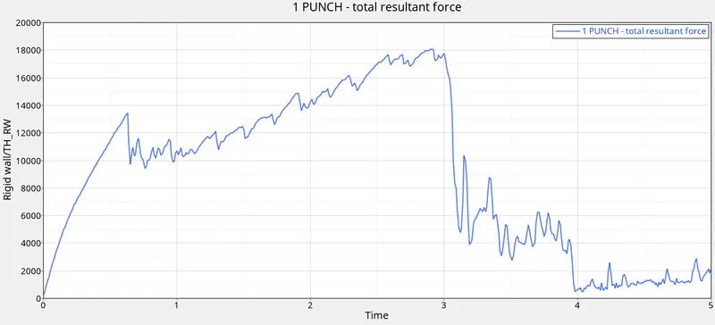
Plot the rigid wall force graph by selecting variables as rigid wall and resultant force and then apply. the graph is plotted.

Case 7- change the material card to Law 27:

In this case, we need use the file which has changed to law 27 material card. Now import that file. verify the material card assigned as LAW 27. Change the shell properties in property card to recommended shell properties as Ishell=24, Ismstr=2, Ish3n=2, Ithick=1, Iplas=1. after changing the properties, run the simulation as follows same procedure in previous case.

 

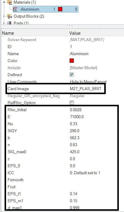
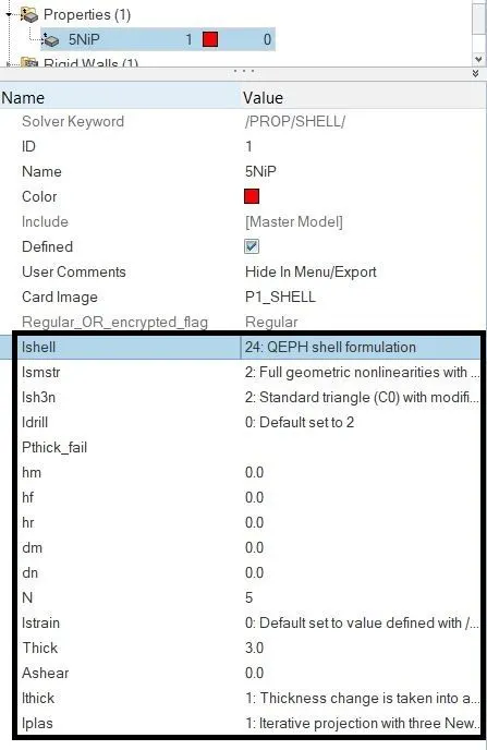
Now open 0001.out file in path directory to check the energy error, mass error, internal energy, kinetic energy etc.,

The obtained last cycle values are 

energy error=0.8%

kinetic energy=65.00 KJ

internal energy=0.2954E+05 KJ

mass error=0

total no.of.cycles=49508

Elapsed time=138.83 s

Now switch the panel to hyperview. Load the h3d file. assign the  parameters result type as von mises, selection as components, averaging method as simple and then apply to run the animation. the animation shown below, The elements will break due to brittle material property.

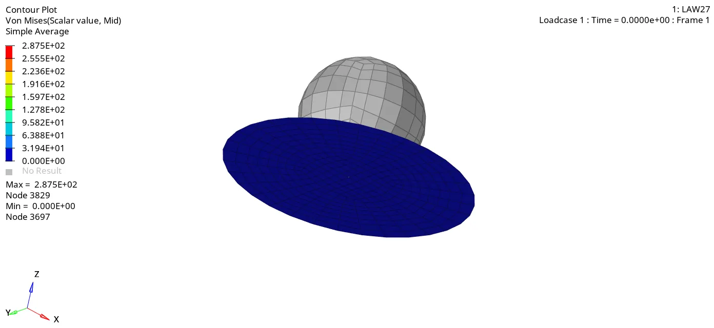
The next step is to plot the energy graphs by switching the panel to hypergraph 2D panel, Now load the T01 file.

Plot the rigid wall force graph by selecting variables as rigid wall and resultant force and then apply. the graph is plotted. The graph reaches to peak value at the time of impact after that decreases gradually.

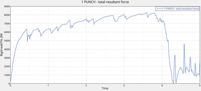
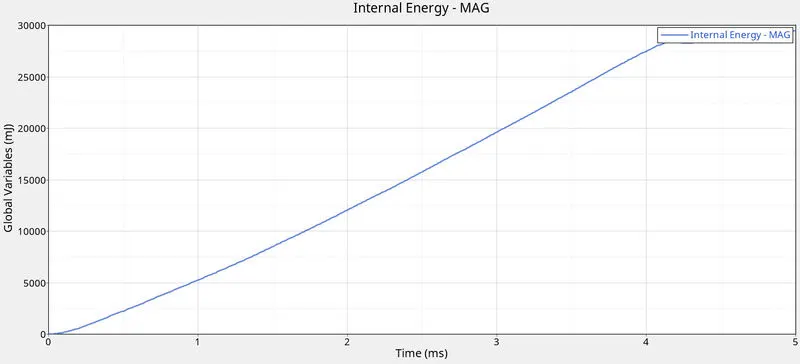
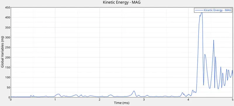
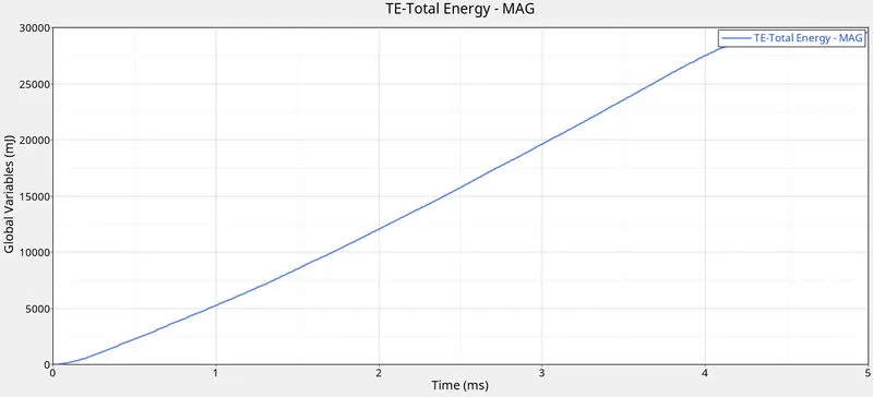
Now plot the energy graphs by change the variables as internal energy, kinetic energy, hourglass energy, total energy and select apply to plot the graphs.

The internal energy is plotted as shown below,

The kinetic energy is plotted as shown below,

Hourglass energy is constant due to the presence of recommended properties.

The total energy increases due to increasing of internal energy and kinetic energy. the graph is plotted below,

Results:

Comparing all the cases explained above

Cases	Energy error	Mass error	No.of.cycles	simulation time	Conditions of elements under more stress
Case 1- Run base simulation without any changes(law 2)	0.8%	0	49380	139.41 s	the elements are deleted
Case 2- changing the values in failure card (law 2)	4.1%	0	49217	149.43 s	elements undergo cracking and then deleted
Case 3- Deleting the failure card (law 2)	0.8%	0	49408	139.29 s	the elements are deleted
Case 4-Deleting the EPS_max value from the material card (law 2)	3.0%	0	48737	133.32 s	cannot be deleted to deletion of failure card & EPS_max value is higher.
Case 5-changing the material card to (Law 1-linear elastic)	1.3%	0	47969	126.37 s	cannot be deleted due to the law behaviour. there is no plastic behaviour takes place.
Case 6- Changing the material card to law 36	-1.2%	0	53159	140.53 s	the elements are deleted
Case 7- change the material card to Law 27	0.8%	0	49508	138.83 s	the elements are deleted

Conclusion:

Finally Done the simulation over the .rad file using variuos cases applied to the given model. plotted the energy graphs and rigid wall force graph for all the cases and compared the results of all the cases.