Week 3.2 - Simulating a 2nd order ODE system of a simple pendulum

clear all 
close all 
clc

% solving the governing eqn of a pendulum
% d^2(theta)/dt^2 + b/m d(theta)/dt + g/L sin(theta) = 0

%inputs
b=0.5;                    %damping coefficient
g=9.8;                    % acceleration due to gravity
m=1;                      % mass of the ball 
l=1;                      % length of the pendulum
t= linspace(0,20,1000);   % the time interval from 0 to 20s is divided equally into 
                            1000time steps
theta_0=[0;3];            % initial conditions for angular displacement and velocity


% solving the ODE using ode45 solver 
% the ode45 solver returns the solution of two first order DEs and time 

[time,results]=ode45(@(t,theta)pendulum_func(t,theta,b,g,m,l),t,theta_0);
    
x0=0;                    % fixed end of the pendulum system
y0=0;

%creating a uncompressed file pendulum_animation.avi and assigning it to videofile

videofile=VideoWriter('pendulum_animation.avi','Uncompressed AVI');

open(videofile);

ct=1;                     % loop counter variable
figure(2)
for i=1:length(t)        % for loop to calculate the position of the ball at each time 
                          
  x1=l*sin(results(i,1));  
  y1=-l*cos(results(i,1)); % the position of the moving end is the angular displacement 
                             at that particular time 

%plotting
plot([x0 x1],[y0 y1])            % plotting the string(line) of pendulum system
hold on 
plot(x1,y1,'.','markersize',40)  % plotting the bob 
hold off                         % to hold from creating multiple overlapping images
axis([-1,1,-1,0])
pause(0.01)
W(ct) = getframe(gcf);           % capturing the current figure using get frame cmd
writeVideo(videofile,W(ct));     % All the frames that are being captured are stitched 
                                   into a video

ct=ct+1;                         % loop variable incrementation

end

close(videofile);


----------------------------------------------------------------------------------------
% definition of the pendulum_func which is used while solving the ode using ode45 solver
% second order DE is broken down into two first order DEs
% first DE is theta_dot(1)= theta(2)
% second DE is theta_dot(2)= -(b/m)*theta(2)-(g/l)*sin(theta(1))


function theta_dot = pendulum_func(t,theta,b,g,m,l)
  
  theta_dot=zeros(2,1);
  theta_dot(1)= theta(2);
  theta_dot(2)= -(b/m)*theta(2)-(g/l)*sin(theta(1));

  end

To simulate the pendulum system , the governing equation d^2(theta)/dt^2 + b/m d(theta)/dt + g/L sin(theta) = 0 is solved.

The governing Differential equation consists of various constants

g = gravity in m/s2,

L = length of the pendulum in m,

m = mass of the ball in kg,

b=damping coefficient.

First , values for these constants are taken as inputs.

L=1 metre,

m=1 kg,

b=0.05.

g=9.81 m/s2.

We are interested to simulate the pendulum system between 0 to 20s . So , the time between 0 to 20s is divided into 1000 equal time steps by using linspace .

To solve the DEs we require the initial conditions of the system which are given as angular displacement = 0 and angular velocity = 3 rad/s (at time = 0).

To solve the second order DE of pendulum system , we break it down into two first order DEs as the ode45(built in solver) solves first order DEs.

[TOUT,YOUT] = ode45(ODEFUN,TSPAN,Y0) syntax of the ode45 solver.

[time,results]=ode45(@(t,theta)pendulum_func(t,theta,b,g,m,l),t,theta_0)

As the second order DE is broken into two first order DEs , 'pendulum_func' function is used which takes in inputs t,theta,b,g,m,l and is defined as 2x1 matrix

theta_dot(1)= theta(2);
theta_dot(2)= -(b/m)*theta(2)-(g/l)*sin(theta(1));

All of the required information is fed to the ode45 solver i.e, the two first order DEs in the form of a function , initial conditions of the DEs , the time span over which the DEs have to be integrated.

The ode45 solver returns the solution(results) of both the DEs at different time steps(including the time steps).

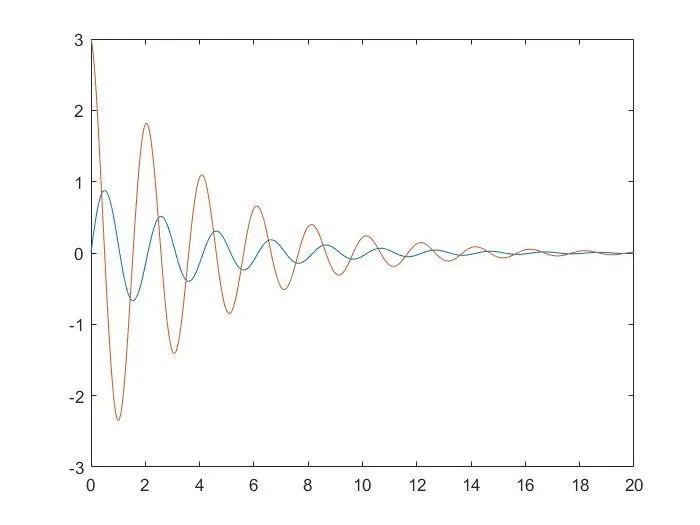
time vs solution of DEs

To simulate the pendulum system first a fixed end needs to be created .

x0=0; y0=0;

At different time values,the bob(moving end) takes different angular displacements as well as angular velocities.

So , 'for ' loop is used to calculate the position of the moving end at different time values/different angular positions(displacments)

x1=l*sin(results(i,1))
y1=-l*cos(results(i,1))

Only the angular displacement (theta ) is required to calculate the position of the bob .So , the first column of the results is used. To only use the first column , the column number is fixed and as i values changes different values can be accessed across the column.

Plotting:

To plot the system , first ,we need to plot the string . plot([x0 x1] [ y0 y1])

Then the bob(moving end) is plotted by changing the size of the marker to 40 . plot(x1,y1,'.','markersize',40)

'Hold on' cmd is used to hold all the current plot and all axis properties.

'Hold off' cmd is used to return to the default mode which erases the previously plotted graphs/images before drawing new plots.

Then the axes are fixed - axis([-1,1,-1,0])

pause(0.01) pauses for 0.01 seconds before continuing . So that we can take a look at the plot.

Animation/GIF :

To create an animation/video of the plots , first , we capture the plot using 'getframe' cmd.By using the loop counter variable ct , plots at different time values are captured .

W(ct) = getframe(gcf)

All the plots that are captured are stored in W array.

Then an uncompressed file pendulum_animation is created and assigned to videofile variable