Week 3.5 - Deriving 4th order approximation of a 2nd order derivative using Taylor Table method
% computing the fourth order approximations for the second order derivative
% f''(x) = a*f(x-2*dx)+b*f(x-dx)+c*f(x)+d*f(x+dx)+e*f(x+2*dx)/dx^2

% f(x) = exp(x)*cos(x)
% analytical_derivative f'(x) = exp(x)*[cos(x) - sin(x)]
% f''(x) = - 2*exp(x)*sin(x)

x=pi/3;

analytical_derivative = - 2*exp(x)*sin(x)

%computing the second order derivative using taylor table central differencing method

%solving the equations obtained from taylors table ax=b
a=[1 1 1 1 1;-2 -1 0 1 2 ; 2 1/2 0 1/2 2;-8/6 -1/6 0 1/6 8/6;16/24 1/24 0 1/24 16/24];

b=[0;0;1;0;0];

z=linsolve(a,b);

dx=linspace(pi/3,pi/300000,200);
f = @(xx,dxx) exp(xx+dxx).*cos(xx+dxx);

%solving the equations ax=b right sided skewed method
a1 = [1 1 1 1 1;0 1 2 3 4;0 1/2 4/2 9/2 16/2;0 1/6 8/6 27/6 64/6;0 1/27 16/24 81/24 256/24];
b1=[0;0;1;0;0];

z1=linsolve(a1,b1);

%solving the equations ax=b left sided skewed method
a2=[1 1 1 1 1;4 3 2 1 0;16/2 9/2 4/2 1/2 0;64/6 27/6 8/6 1/6 0;256/24 81/24 16/24 1/24 0];
b2=[0;0;1;0;0];
z2=linsolve(a2,b2);

for i=1:length(dx)

num_derivative2(i)= (z(1)*f(x,-2*dx(i))+ z(2)*f(x,-dx(i))+z(3)*f(x,0)+z(4)*f(x,dx(i))+z(5)*f(x,2*dx(i)))/dx(i)^2


num_derivative(i) = (z(1)*exp(x-2*dx(i))*cos(x-2*dx(i)) +z(2)*exp(x-dx(i))*cos(x-dx(i)) +z(3)*exp(x)*cos(x) + z(4)*exp(x+dx(i))*cos(x+dx(i))+z(5)*exp(x+2*dx(i))*cos(x+2*dx(i)))/(dx(i).^2);


num_rhs(i) = (z1(1)*f(x,0)+z1(2)*f(x,dx(i))+z1(3)*f(x,2.*dx(i))+z1(4)*f(x,3.*dx(i))+z1(5)*f(x,4.*dx(i)))/(dx(i).^2)


num_lhs(i)= (z2(1)*f(x,-4.*dx(i))+z2(2)*f(x,-3.*dx(i))+z2(3)*f(x,-2.*dx(i))+z2(4)*f(x,-dx(i))+z2(5)*f(x,0))/dx(i).^2


end

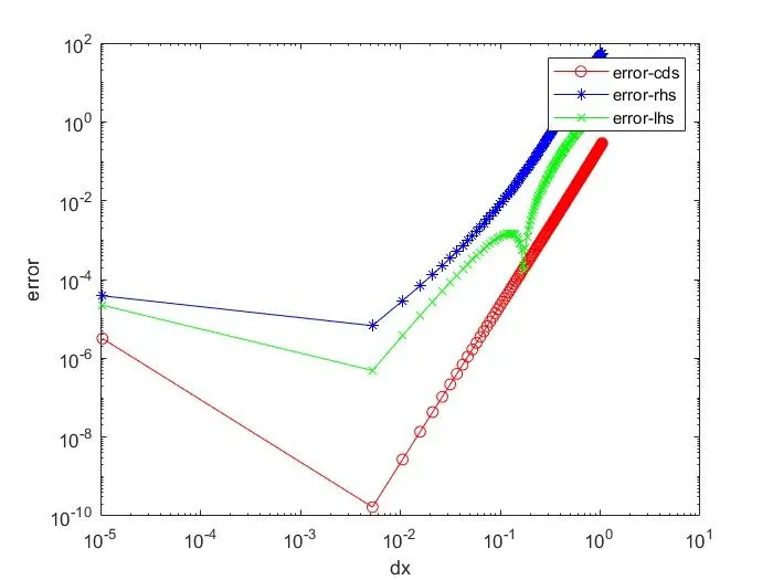
% calculating the error and plotting

error_rhs=abs(analytical_derivative-num_rhs)
error_cds =abs(analytical_derivative-num_derivative2)
error_lhs =abs(analytical_derivative-num_lhs)
loglog(dx,error_cds,'r','Marker','o')
hold on
loglog(dx,error_rhs,'b','Marker','*')
hold on
loglog(dx,error_lhs,'g','Marker','x')
xlabel('dx');
ylabel('error');
legend('error-cds','error-rhs','error-lhs')
To derivate the fourth order approximations of the second order derivative , a numerical scheme/stencil is chosen accordingly.
Fourth order approximation indicates that the information is taken from 4 neighbouring points.
If the neighbouring points lie symmetrical across the point(two on the either side),then it is called central differencing scheme.
If the neighbouring points lie on the right side of the point , then it is called right handed skewed scheme.
If the neighbouring points lie on the left side of the point, then it is called left handed skewed scheme.
The function whose second order derivative is to be compared with the numerical methods is f(x) = exp(x)*cos(x)
analytical first order derivative f'(x) = exp(x)*[cos(x) - sin(x)]
analytical second order derivative f''(x) = - 2*exp(x)*sin(x)
1) central differencing scheme :
Generally, for forward differencing approx. (first order derivative , first order approx.) f'(x) = f(x+dx)-f(x)/dx
f'(x) = a*f(x+dx) + b*f(x)/dx |a=1 b=-1
So we expand this idea and assume coefficients a,b,c,d,e for fourth order approx.
f''(x) = a*f(x-2*dx)+b*f(x-dx)+c*f(x)+d*f(x+dx)+e*f(x+2*dx)/dx^2 ----- (1)
the function at each point is exapanded using taylors approx. method and arranged in a table .
As we are calculating the second order derivative , all the coefficients with f''(x) are equated to 1 and the remaining f(x),f'(x),f'''(x),f''''(x) are equated to zero .
So we get a system of linear equations (5 equations) A*X=B to be solved.They are solved using inbulit solver called 'linsolve' .
Then the coefficients which we had assumed a,b,c,d,e are fed to the above equation (1),and numerical derivative is calculated.
As we are interested to find how the error term varies with change in dx . dx=linspace(pi/3,pi/30000,200) - range operator linspace is used .
'for ' loop is used to calculate the numerical derivative for that particular value of dx. i is the loop counter variable and runs upto the last value of dx array . i = 1:length(dx)
num_derivative(i) = (z(1)*exp(x-2*dx(i))*cos(x-2*dx(i)) +z(2)*exp(x-dx(i))*cos(x-dx(i)) +z(3)*exp(x)*cos(x) + z(4)*exp(x+dx(i))*cos(x+dx(i))+z(5)*exp(x+2*dx(i))*cos(x+2*dx(i)))/(dx(i).^2
A different approach can be used to evaluate the numerical derivative i.e., by defining the function and changing the variables wherever necessary .
f = @(xx,dxx) exp(xx+dxx).*cos(xx+dxx) -- function defined anonymously with variables xx and dxx.
2) skewed right sided scheme :
Similar methodology is followed and numerical derivative(num_rhs)is calculated.
But in this case , all the neighbouring points lie on the right hand side of the point .
3) skewed left sided scheme :
Similar methodology is followed and numerical derivative(num_lhs) is calculated.
But in this case , all the neighbouring points lie on the left hand side of the point .
Similar anonymous function approach is used here as well .