Week 2 Air standard Cycle

Objective: To plot the PV diagram of the otto cycle and compute the thermal efficiency.

Python code:

import math
import matplotlib.pyplot as plt
import numpy as np

def engine_kinematics(bore,stroke,cr,l,start_angle,end_angle):
	# to calculate the volume values at different crank angles for compression and expansion processes
	# v/v_c = 1+0.5(r-1)[R+1-cos(theta)-(R^2-sin^2(theta))^0.5]

	#Inputs

	a=stroke/2
	R=l/a
	theta=np.linspace(start_angle,end_angle,100)

	v_s = (math.pi/4)*pow(bore,2)*stroke
	v_c= v_s/(cr-1)
	v_t=v_s+v_c
	v=[]

	for i in range(len(theta)):
		crank_angle=math.radians(theta[i])


		term1=0.5*(cr-1)
		term2=R+1-math.cos(crank_angle)
		term=pow(R,2)-pow(math.sin(crank_angle),2)
		term3=pow(term,0.5)


		v.append((1+term1*(term2-term3))*v_c)
		

	return v

# To plot the PV diagram of otto cycle by computing the state variables 
#Inputs
gamma=1.4

#Initial state variable(assumption)
p1=101325
t1=500

# To compute the volume at state point 1 using the geometry

#vol of the cylinder = swept volume + clearance volume
# swept volume = the volume covered by the piston while moving from TDC to BDC = pi/4* dia of cylinder^2 * length of the cylinder
# clearance volume = swept vol/compression ratio -1
# Geometrical inputs
bore=0.1
stroke=0.1
cr=12
l=0.15

v_s = (math.pi/4)*pow(bore,2)*stroke
v_c= v_s/(cr-1)
v1=v_s+v_c

# state point 2
v2=v_c
p2=(p1*pow(v1,gamma))/pow(v2,gamma)
#to compute t2 using the ideal gas relation p2*v2/t2 = p1*v1/t1
rhs= (p1*v1)/t1
t2=p2*v2/rhs

# to compute the volume values for different crank angles in compression process
v_compression=engine_kinematics(bore,stroke,cr,l,180,0)
const=p1*pow(v1,gamma)
p_compression=[]

for j in range(len(v_compression)):
	p_compression.append(const/pow(v_compression[j],gamma))
	
#state point 3
v3 = v2
t3 = 2300 # assumption

#to compute p3 using ideal gas relation p3*v3/t3 = p2*v2/t2
rhs1=p2*v2/t2
p3 = rhs1 *t3/v3

# to compute the volume values for expansion process
v_expansion=engine_kinematics(bore,stroke,cr,l,0,180)
const1=p3*pow(v3,gamma)
p_expansion=[]

for w in range(len(v_expansion)):
	p_expansion.append(const1/pow(v_expansion[w],gamma)) 

#state point 4
v4 = v1 

#to compute the pressure using the adiabatic relation pv^gamma = constant | p3v3^gamma =p4 v4^gamma
p4= p3*pow(v3,gamma)/pow(v4,gamma)

# to compute the temp using the ideal gas relation p3v3/t3 = p4v4/t4| t4 = p4v4/rhs2
rhs2= p3*v3/t3
t4= p4*v4/rhs2

plt.plot([v2,v3],[p2,p3])
plt.plot([v4,v1],[p4,p1])
plt.plot(v_compression,p_compression)
plt.plot(v_expansion,p_expansion)
plt.xlabel('volume')
plt.ylabel('pressure')
plt.title('p-v diagram')
plt.show()

# To compute the thermal efficiency of the otto cycle

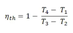
eff = 1 - (t4-t1)/(t3-t2)
print("the thermal efficiency of the otto cycle is {0}".format(eff) )

Explanation:

1. First, we compute the state variables by assuming the values at initial state point 1 and using the adiabatic relation pv^gamma = constant and ideal gas law pv=nrt.

2. In the first process i.e, from state point 1 to 2, adiabatic compression takes place.

In the second process i.e, from state point 2 to 3, constant volume heat addition or combustion takes place.

In the third process i.e, from state point 3 to 4, adiabatic expansion takes place.

In the fourth process i.e, from state point 4 to 1, constant volume heat rejection takes place.

3. In the compression process, the piston travels from BDC to TDC, so the volume at the start of the compression stroke(state point 1) is the volume of the cylinder at BDC, which can be computed by adding the clearance volume and swept volume.

4. Similarly, the other properties at different states are computed.

5. But when the state points are connected, the path between the compression and expansion processes is linear, which is not practical.

6. So, the volume values for different crank angles are calculated using the relation mentioned below, and then the other properties are calculated using the adiabatic relation.

7. A function ' engine_kinematics' is defined which takes bore, stroke, connecting rod length, compression ratio, and starting and ending crank angles as input and returns the volume array for different crank angles.

8. This function is called, to compute the volume array between state points 1 and 2, and, 3 and 4.

9. Finally, the state points, volume, and pressure arrays are plotted. And also the thermal efficiency is calculated and printed.

Output:

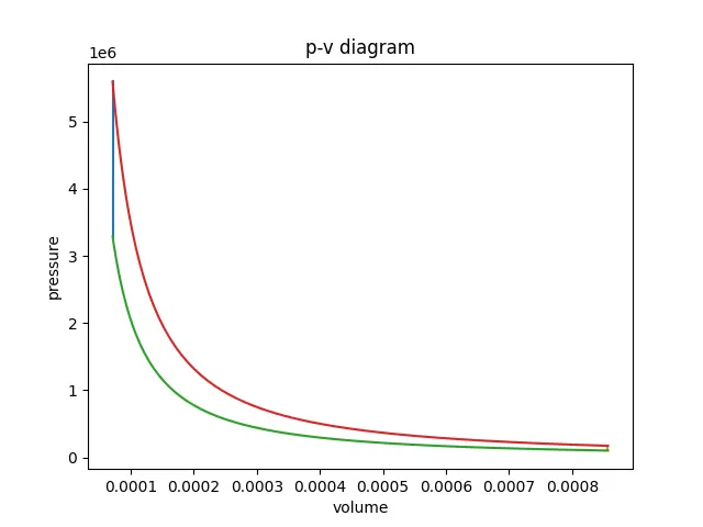
The thermal efficiency of the otto cycle is 0.6238