Week-7 Simulating Fluid Sloshing effect inside a Gear-box

Aim :

1. To perform fluid sloshing simulations in the gearbox to visualize the reach of the fluid over the gear teeth.

2. To implement dynamic meshing methods and user-defined functions for this application.

Introduction :

Fluid sloshing :

In fluid dynamics, slosh refers to the movement of liquid inside another object. It is caused by any disturbance to partially filled liquid containers. Depending on the type of disturbance and container shape, the free liquid surface can experience different types of motion including simple planar, nonplanar, rotational, irregular beating, symmetric, asymmetric, quasi-periodic, and chaotic. When interacting with its elastic container, or its support structure, the free liquid surface can exhibit fascinating types of motion in the form of energy exchange between interacting modes.

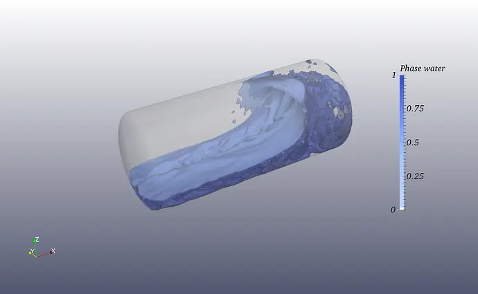
The sloshing effect of the liquids is considered to be an important factor in areas such as cargo ships (tankers) that transport petroleum liquids or other liquids (water inside of ballast tanks). Sloshing can produce big problems so is essential to apply prevention measures. For example in water ballast tanks, the sloshing motion of seawater inside ballast tanks will bring large fluid pressures and impact loads, which might destroy the structure of tanks. Moreover, it may create a torque that may cause the vehicle to tip over.

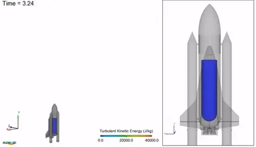
A large fraction of the mass of a satellite is liquid propellant at/near the Beginning of Life (BOL), and slosh can adversely affect satellite performance in several ways. For example, propellant slosh can introduce uncertainty in spacecraft attitude.

Fluid sloshing in the above cases is undesired. But in the case of lubrication of gear teeth, fluid sloshing is very helpful.

Dynamic Meshing:

Normal Meshing is done on geometries that are physically not going to change. For most CFD simulations the physical geometry does not change with time, and a steady mesh will then generally be the appropriate choice. Dynamic meshing refers to situations in which the computational grid changes dynamically during the run of the CFD simulation. This opens up the possibility to simulate flows where the geometry changes with time.

The dynamic mesh model can be used to move the boundaries of a cell zone relative to other boundaries of the zone, and to adjust the mesh accordingly. The boundaries can move rigidly concerning each other (linear/rotational) and/or deform. The motion of the boundaries can be rigid, such as pistons moving inside an engine cylinder, or deforming such as the elastic wall of a balloon during inflation. To use the dynamic mesh model, the starting volume mesh should be provided and the description of the motion of moving zones in the model. Ansys Fluent allows describing the motion using either boundary profiles, UDFs, or six degrees of freedom solver.

User Defined Functions:

UDFs allow you to customize ANSYS FLUENT to fit your particular modeling needs. UDFs can be used for a variety of applications. A user-defined function, or UDF, is a function that you program that can be dynamically loaded with the ANSYS FLUENT solver to enhance the standard features of the code. Some examples include customization of boundary conditions, material property definitions, surface and volume reaction rates source terms in ANSYS FLUENT transport equations, source terms in user-defined scalar (UDS) transport equations, diffusivity functions, etc. In this case, a UDF is defined to give motion to the gears.

UDFs are written in the C programming language using any text editor and the source code file is saved with a .c extension (e.g., myudf.c). One source file can contain a single UDF or multiple UDFs, and you can define multiple source files.

In any CFD analysis, the workflow that is followed is

Setting up the geometry ----> Meshing ----> setting up the solver ---->solving ---->post-processing results

step-1 Setting up the geometry :

First, the pre-designed gearbox which consists of two gears in the housing is imported to the Spaceclaim module.

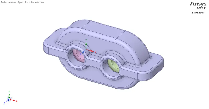
3D model of the gearbox

As we are interested in simulating the fluid flow inside the gearbox, the fluid volume is extracted by selecting all the edges which make up the volume.

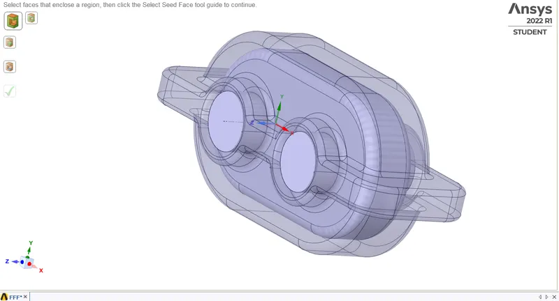
After volume extraction

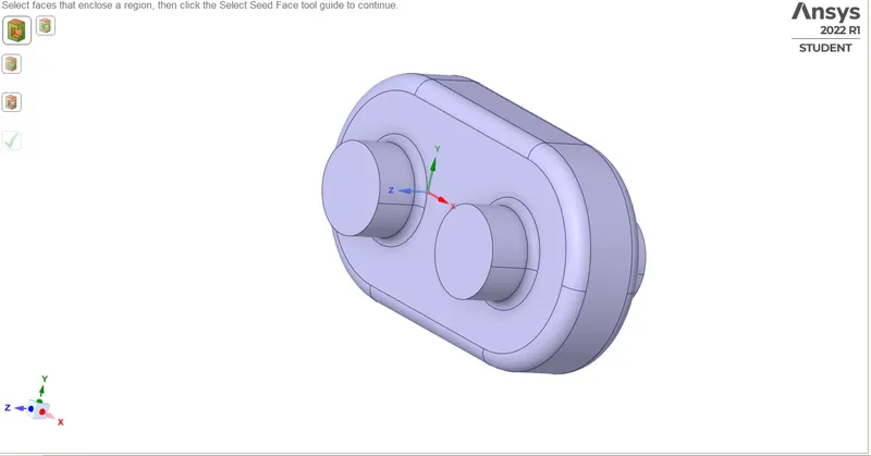
fluid volume

As we are interested in performing a 2D flow simulation inside the gearbox, the center plane is extracted by splitting the fluid volume into two parts across the z-axis.

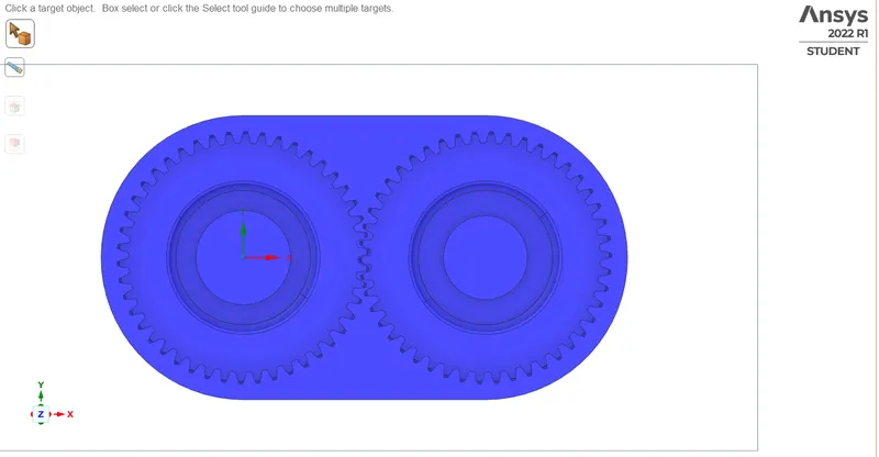
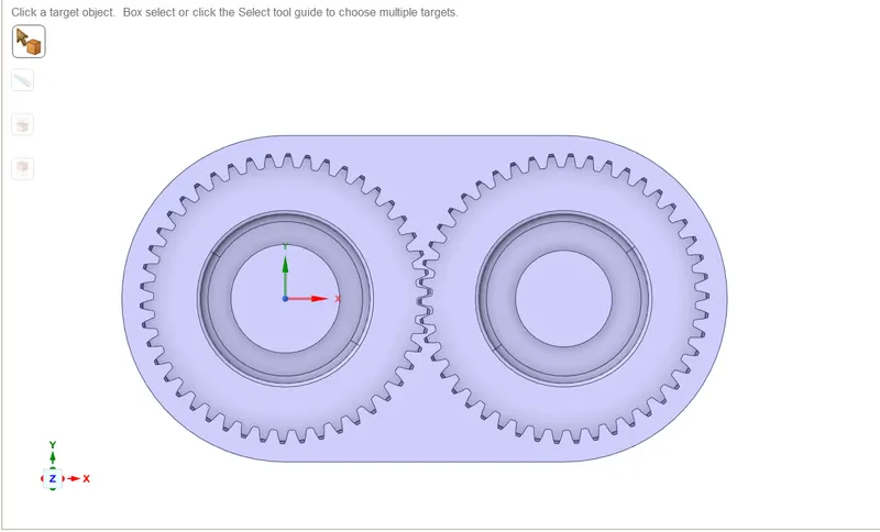
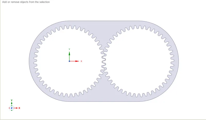
2D plane of the gearbox

Now, we can further proceed to mesh the plane.

step-2 Meshing :

Meshing is the process of generating a grid i.e, dividing complex geometries into elements that can be used to discretize a domain.

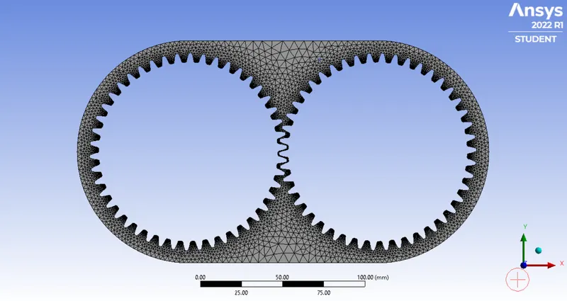
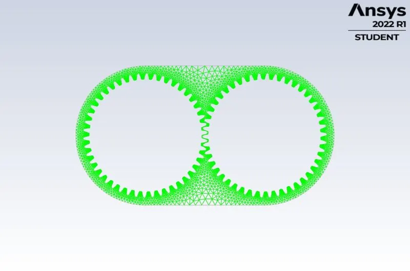
The mesh generated is an automated mesh consisting of triangular elements. To check the quality of the mesh, the mesh metrics option is changed to element quality in mesh settings.

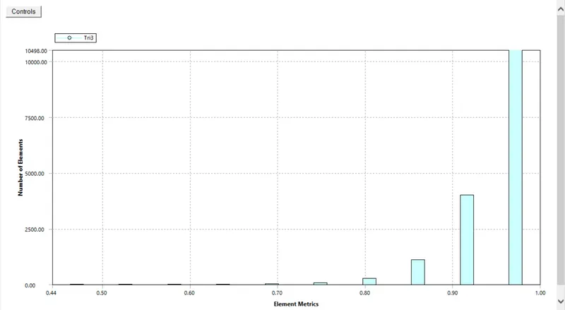
Most of the elements fall in between 0.90 and 1 (1 being the perfect Tri3-shaped element)and the least number of elements fall below 0.40, which is perfectly fine.

Then the boundaries are defined by selecting the edges of the gear and naming them accordingly.

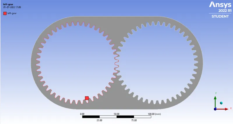
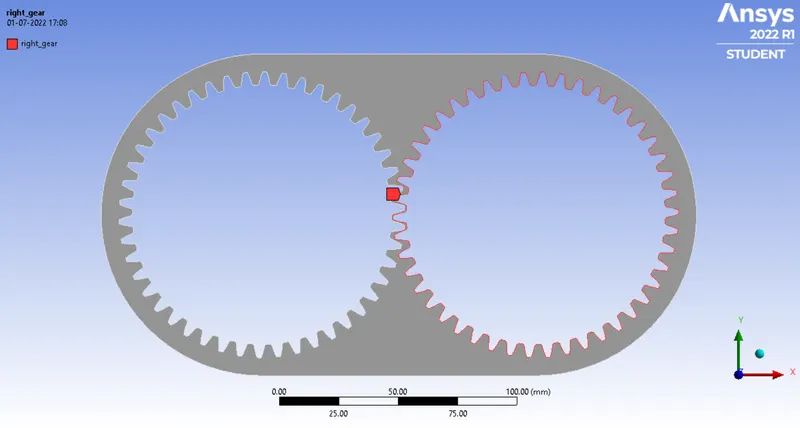
Now, we can proceed further to set up the flow physics.

step-3 Setting up the solver in Ansys FLuent:

In this step, we define parameters like initial and boundary conditions, materials used, time steps(for transient), turbulence model, etc., which captures the physics to be simulated.

First, we set up the physics by choosing the pressure-based solver which was particularly designed for low-speed incompressible flows(low Mach number). The gravity field is applied in the negative y-direction(-9.81m/s2).

The transient solver is checked. For this approach, transient state analysis is implemented as the physics that evolves, is a function of time.

As we are dealing with two phases(air and engine oil), multi-phase modeling i.e, the Volume of fluid model with implicit method, has to be applied.

k-epsilon realizable turbulence model with enhanced wall treatment is selected.

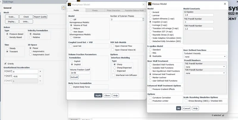
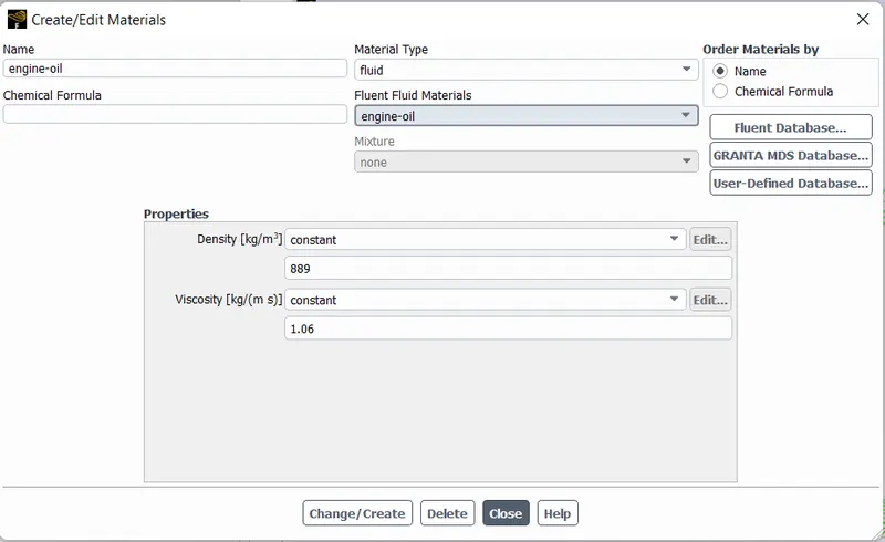
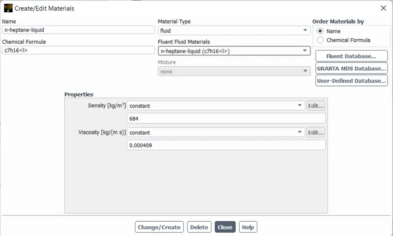
Then the materials- engine oil, and n-heptane, are copied from the fluent database and assigned as the secondary fluid(s) in the multiphase model.

Now, the dynamic mesh is set up by checking all the mesh methods i.e, Smoothing, layering, and remeshing.

Smoothing is used to adjust the mesh of a zone with a moving and/or deforming boundary, the interior nodes of the mesh move, but the number of nodes and their connectivity does not change.

Dynamic layering is used to split or merge cells adjacent to any moving boundary.

When the boundary displacement is large compared to the local cell sizes, the cell quality can deteriorate if only mesh smoothing is used. This may result in negative cell volumes and consequently, will lead to convergence problems.To circumvent this problem, ANSYS collects the group of cells that violate skewness or size criteria and locally remeshes the group of cells.

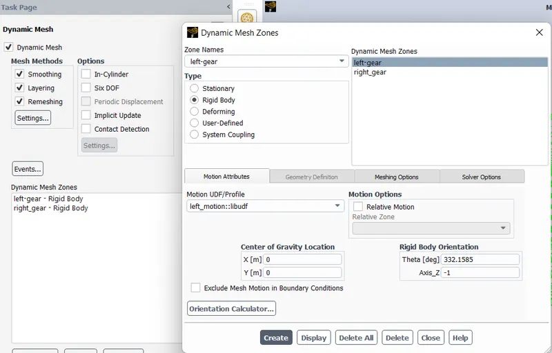
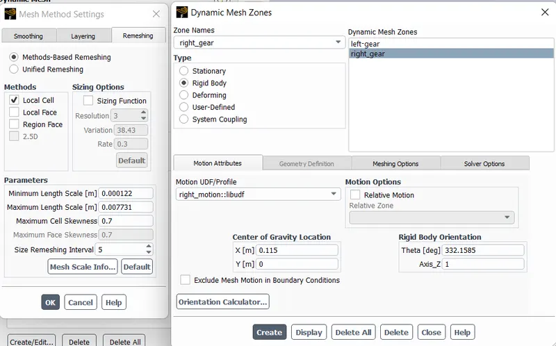
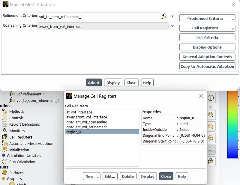
Then, the region that is made up of engine oil/n-heptane is created, and occupies 20% or 30% of the fluid volume.

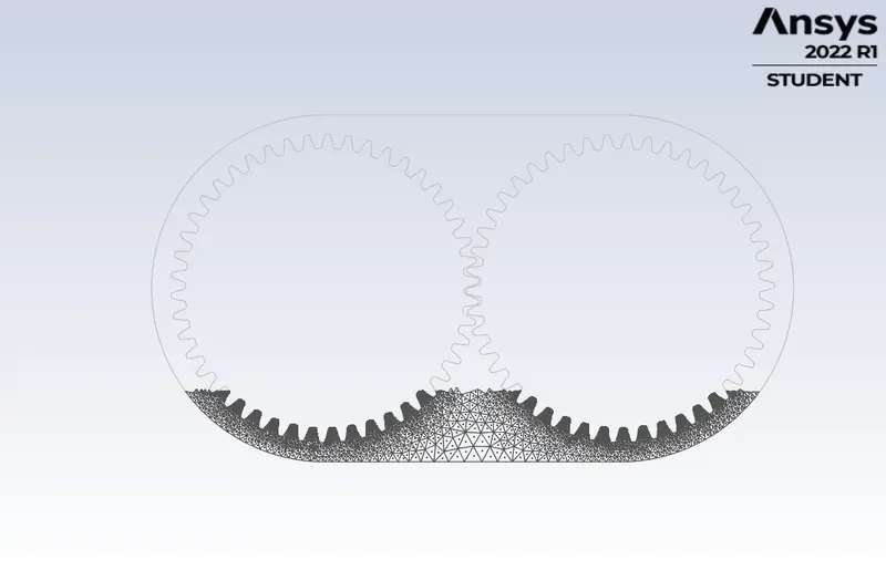
20% immersion of engine oil/n-heptane

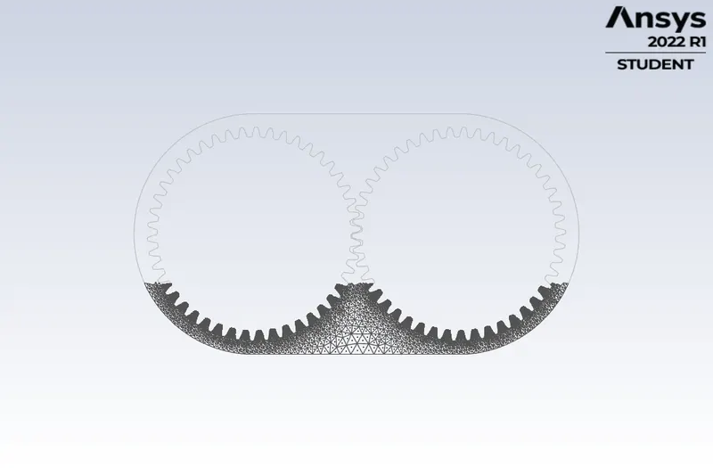
30% immersion of engine oil/n-heptane

Now, the User-defined function to describe the motion of the moving zones/gears is loaded.

#include "udf.h"

DEFINE_CG_MOTION(right_motion, dt, vel, omega, time, dtime)
{
	vel[0] = 0.0;
	vel[1] = 0.0;
	vel[2] = 0.0;

	omega[0] = 0.0;
	omega[1] = 0.0;
	omega[2] = 2.0e2; /* [rad/s]*/
}
DEFINE_CG_MOTION(left_motion, dt, vel, omega, time, dtime)
{
	vel[0] = 0.0;
	vel[1] = 0.0;
	vel[2] = 0.0;

	omega[0] = 0.0;
	omega[1] = 0.0;
	omega[2] = -2.0e2; /* [rad/s]*/
}

Hybrid initialization is chosen for initializing the domain. Hybrid Initialization is a collection of recipes and boundary interpolation methods. It solves the Laplace equation to produce a velocity field that conforms to complex domain geometries, and a pressure field that smoothly connects high and low-pressure values in the computational domain.

After initializing the domain, we patch the region that we had previously created as the engine oil/n-heptane.

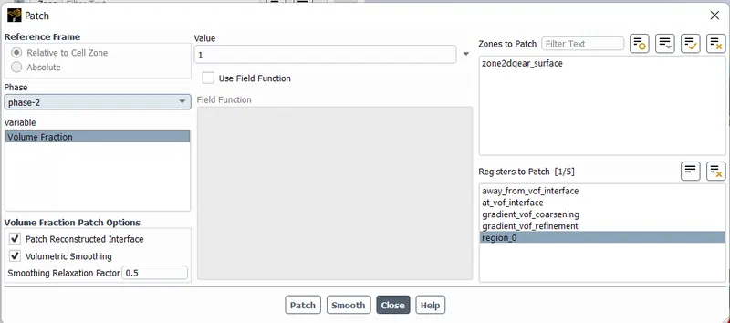
The time-step size is chosen as 1e-4 and the solver is run for 10000 timesteps.

Results:

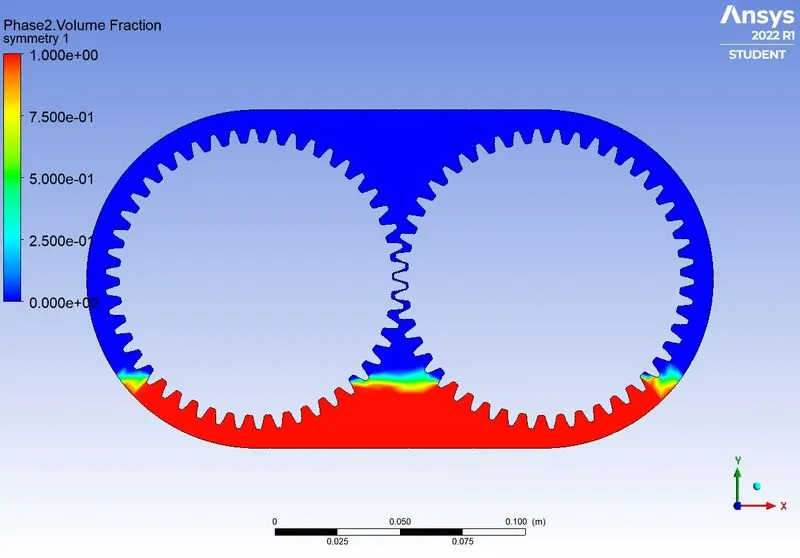
initial contour

Residuals :

case1 - 20% engine oil immersion

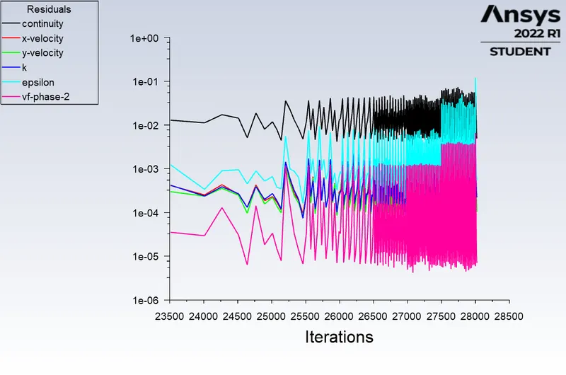
case2 - 20% n-heptane liquid immersion

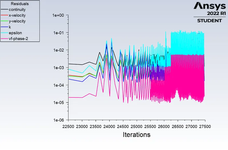
case3 - 30% engine oil immersion

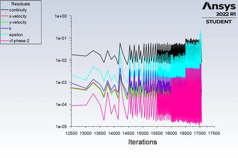
case4- 30% n-heptane liquid immersion

Comparison of volume fraction contours at different time-steps:

20% immersion of engine oil

20% immersion of n-heptane liquid

30% immersion of engine oil

30% immersion of n-heptane liquid

Animation video:

case1 - 20% engine oil immersion

case2 - 20% n-heptane liquid immersion

case3 - 30% engine oil immersion

case4- 30% n-heptane liquid immersion

Observation and Conclusion :

1. At 20% immersion both the fluids - engine oil and n-heptane liquid, reached the same gear teeth.

2. At 30% immersion both the fluids - engine oil and n-heptane liquid, reached the same gear teeth.

3. On comparing the 20% immersion case and 30% immersion case of engine oil and n-heptane liquid, at the same time step (100th-time step), the 30% immersed fluid had a better reach. So, the greater the volume of immersed liquid, the better the reach/spread.