Week 4.2 - Linear Convection for varying timesteps
Aim :
To solve the one-dimensional linear convection equation which partly resembles the governing momentum equation in Matlab. And to analyze how the solution changes with changing the size of time steps.
Matlab code :
Writing a function that takes the input argument as the size of the time step to analyze how the results vary with the size of the time steps.
Main code:
% taking dt as input and solving for velocity profiles for every timestep
clear all
close all
clc

L=1;
n=80;
x=linspace(0,L,n);
dx=x(2)-x(1);

%initial velocity profile for plotting
    u=ones(1,n);
    n_start=0.1/dx + 1;
    n_end=0.3/dx + 1;
    u(n_start:n_end)=2;
    u_initial= u ;


nt=80;

% using tic toc cmd to calculate the run time of each simulation
tic;
[x1,uold1]=velcalc(1e-4);
t1= toc;

tic;
[x2,uold2]=velcalc(1e-3);
t2= toc;

tic;
[x3,uold3]=velcalc(1e-2);
t3= toc;

tic
[x4,uold4]=velcalc(1e-1);
t4=toc;


%plotting
plot(x,u_initial,'k',LineWidth=2);
hold on
plot(x1,uold1,'b',LineWidth=2);
 hold on
plot(x2,uold2,'y',LineWidth=2);
hold on
plot(x3,uold3,'r',LineWidth=2);
hold on
plot(x4,uold4,'g',LineWidth=0.1);
axis([0 1 0 2])
legend('initial velocity profile','timestep1 - 1e-4','timestep2 - 1e-3','timestep3 - 1e-2','timestep4 - 1e-1')
title('effect of time step')


total_time_of_simulation=[t1 t2 t3 t4];
h=categorical({'1e-4','1e-3','1e-2','1e-1'});
figure(2)
bar(h,total_time_of_simulation,'g')
xlabel('time step');
ylabel('simulation time');
title('simulation time');
function code:
velcalc function takes dt as the input and returns x and velocity final array(uold) values as output to plot .
function [x,uold] = velcalc(dt)

    L=1;
    n=80;
    c=1;
    x=linspace(0,L,n);

    % creating the domain
    dx=x(2)-x(1);           % element size
    nt=0.4/dt;             % number of time steps

    %initialize arrays
    u=ones(1,n);
    n_start=0.1/dx + 1;
    n_end=0.3/dx + 1;
    u(n_start:n_end)=2;
    u_initial= u ;

    %Applying boundary conitions
    u(1)=1;
    uold=u;       % assigning uold as the initial array


    %solving the equation ( time loop)
    for j=1:nt
        for i=2:n % space loop


            u(i) = -c*dt/dx*(uold(i)-uold(i-1))+uold(i);

        end

        uold = u; % updating the old values


        co = u*(dt/dx);


    end
explanation of the code :
1. First, the domain is created. Then the initial and boundary conditions are defined.
2. With the information from the initial velocity profile, velocity profiles at each time step are computed using for loop(space and time loop).
3. The initial array is assigned as uold, as we are calculating the velocity for the current time step, and then after calculating for the current time step we assign it as uold.
4. using the func 'velcalc' which takes input dt and returns velocity array at the final time step as mentioned above.
5.The main code consists of calculating the final velocity profile at different time steps - 1e-4,1e-3,1e-2,1e-1.
6. The final velocity profiles at different time steps are plotted with different line specifications like color, width and compared with the initial velocity profile(i.e a square wave).
7. The run time of each velocity profile calculation at different time steps is calculated using 'tic toc' cmd.
8. The tic toc is basically like a stopwatch, when a tic is used the timer runs and the toc is used to stop the timer. So, tic and toc are used before and after each final velocity calculation.
9. A bar graph is plotted between run time/simulation time which we stored in t1,t2,t3,t4, and different time steps.
Results/Plots :
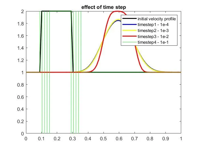
initial and final velocity profiles at different time steps
Explanation of the plot behavior :
Numerical diffusion:
Numerical diffusion refers to the amplitude damping of the numerical solution as compared to the exact solution. This occurs as we are ignoring the terms (truncation error) in forward and backward differencing schemes for time and space derivatives.

1.The RHS is the truncation error for convection equation, v is the CFL number (v) [v= u * dt/dx] ,the coefficient of ∂^2 u /∂x^2 i.e, (a*dx)/2*(1-v) is called the diffusivity coefficient
2. As the size of the time step(dt) increases, the CFL number(v) also increases, but (1-v) decreases in a positive range (up to a maximum of v=1). So the diffusivity coefficient decreases(positive magnitude) which makes the velocity profile diffuse less.
3.1e-2 time step has the least diffusivity because the CFL number is almost 1.
(when v<1 the diffusivity coefficient is positive and has a diffusive effect.)
4. But when the time step is 1e-1 (largest time step), the CFL number > 1 . So, the diffusivity coefficient becomes negative and the solution blows up.
( when v>1 the diffusivity coefficient becomes negative and has an amplifying effect and is the cause of instability.)
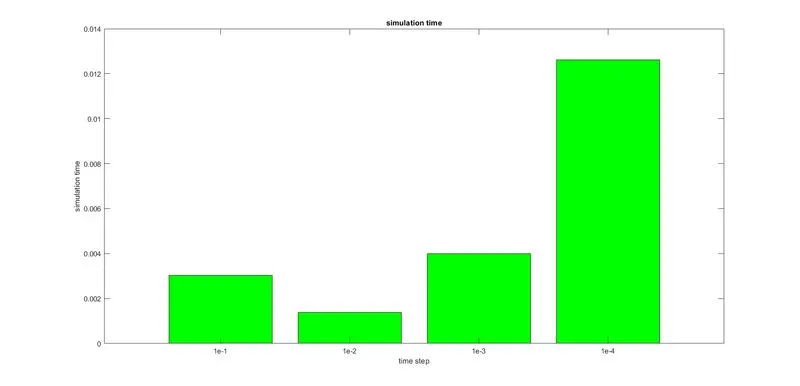
bar graph showing run time/simulation time for various sizes of time steps
Explanation of the bar graph :
As the size of the time step decreases, the number of time steps increases(to keep the simulation run time 0.4s constant), and computing velocity array at each time step increases the run time (or) time taken for the calculation. So we can observe that the 1e-4 time step has a greater run time and run time decreases accordingly with an increase in the size of the time step. But, the run time for the 1e-1 time step is greater than 1e-2 which is because the solution blows up.