Week 3 - Solving second order ODEs

Objective: To solve the second order ODE that governs the pendulum using the odeint function, and creating animation of the pendulum.

Problem Statement : The differential equations are the equations that are used to predict the behaviour of bodies. And solving them is one of the most important aspect. The governing equation that predicts the motion of pendulum is a second order ODE.

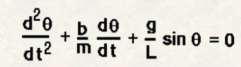
This equation conveys that the angular displacement varies with respect to time. And by changing the values of the parameters, the angular displacement might vary more or less.

python code:

# to solve the odes governing the pendulum motion 
import numpy as np
from scipy.integrate import odeint
import math
import matplotlib.pyplot as plt

# theta function

def sample(theta,t,b,m,g,l):
	theta1=theta[0]
	theta2=theta[1]
	dtheta1_dt=theta2
	dtheta2_dt=-(b/m)*theta2-(g/l)*math.sin(theta1)
	dtheta_dt=[dtheta1_dt,dtheta2_dt]

	return (dtheta_dt)

# inputs 

#damping coeff
b=0.05
#mass of the bob
m=1
#acceleration due to gravity
g=9.81
#length of the pendulum
l=1
# time array
t=np.linspace(0,10,100)

#initial array
theta_in = [0,5]

#solving the ODE using odeint

theta=odeint(sample,theta_in,t,args = (b,m,g,l))
#plotting
plt.plot(t,theta[:,0])
plt.plot(t,theta[:,1])
plt.xlabel('time[s]')
plt.ylabel('angular displacement[radians]')
plt.title('second order ODE')
plt.show()

theta1=theta[:,0]

# plotting pendulum animation
x0=0
y0=0

ct=0
for i in range(len(theta1)):
	x1=l*math.sin(theta1[i])
	y1=-l*math.cos(theta1[i])
	ct=ct+1
	
	filename=str(ct)+'.png'
	plt.figure(ct)
	plt.plot([x0,x1],[y0,y1],linewidth=2)
	plt.plot(x1,y1,'o','marker',markersize=20,color='k')
	plt.plot([2,2],[0,0],linewidth=5)
	plt.xlim(-2.5,2.5)
	plt.ylim(-2.5,2.5)
	plt.title('pendulum animation')
	plt.savefig(filename)
	

explanation of the code:

1. First, the parameters like damping coefficient, mass of the bob, acceleration due to gravity, length of the pendulum, the inital values of the differential equations, and the time array over which the angular displacement should be integrated are specified.

2. Then the second order ODE is broken down into two first order ODEs

`(d(theta_1))/(dt)=theta_2`

`(d(theta_2))/dt=-(b/m)theta_2-(g/L)sin(theta_1)`

And these two differential equations are returned by a function ' sample' which takes inputs theta (solution of the differential equations), time, b, m , g,and l.

3. 'odeint' is used to solve the first order ODEs which takes inputs - the differential equations, initial values of the two differential equations, time array over which the DEs have to be integrated over, and the arguments- b, m ,g and l.

4. The solution of these two ODEs is stored in theta array, which has two solution sets, one is the solution of the first ODE

`(d(theta_1))/(dt)=theta_2` which gives the values of angular displacement.

5. On the other hand, the second set is the solution of the second ODE `(d(theta_2))/dt=-(b/m)theta_2-(g/L)sin(theta_1)` which gives the rate of change of angular displacement ie, angular velocity.

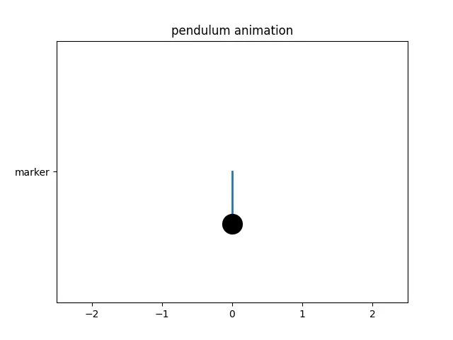
6. Then, a plot is created between the angular displacement vs time and angular velocity vs time. To plot the animation, a base point x0,y0 is created and the other end is moving wrt theta , which is changing as a function of time. x1=l*sin(theta) y1=-l*cos(theta). A for loop is used as theta is an array and a loop variable ct is used to save the figures.