Week 3 - External flow simulation over an Ahmed body.
Aim :
1. To perform external flow simulations over the Ahmed body.
2. To perform a grid independency study.
3. To understand the importance of the Ahmed body and the physics behind it.
Introduction :
Optimized external car aerodynamics is necessary to achieve efficient vehicles with minimized fuel consumption, CO2 emissions, and noise while keeping good driving stability. Steadily increasing computer power has been raising the importance of simulating the external aerodynamics of vehicles and computing the corresponding aerodynamic characteristic numbers. The Ahmed model was created by SR Ahmed in 1984 and was designed to be a simple geometry that was capable of replicating complex flow structures involved in the flow past an automobile. It has evolved into a benchmark problem for CFD solvers aiming to capture accurately the flow features of an automobile. This model is also used to describe the turbulent flow field around a car-like geometry. When the numerical model is validated, it is used to design new models of the car.
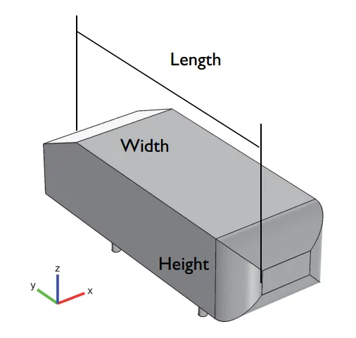
Ahmed body
The flow region presents the major contribution to a car's drag, and poses severe problems to numerical predictions and experimental studies as well, as the wake flow behind the car. The location at which the flow separates determines the size of the separation zone, and consequently the drag force.
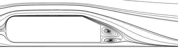
recirculation zone in the wake region
In any CFD analysis, the workflow that is followed is
Setting up the geometry ----> Meshing ----> setting up the solver ---->solving ---->post-processing results
step-1 Setting up the geometry :
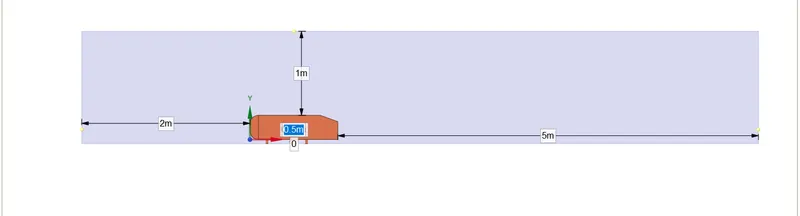
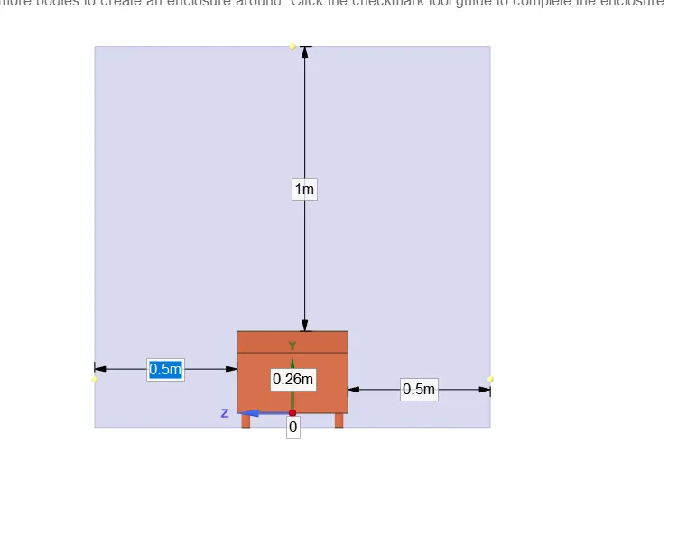
First, the pre-modeled Ahmed body is imported into Spaceclaim to create a domain(wind tunnel) around it by using the enclosure feature. The dimensions of the 3D domain are shown below:
front view of the domain
side view of the domain
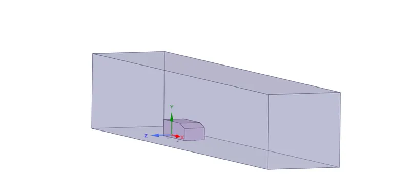
3D view of the domain
When using the enclosure feature, it automatically deletes the body's volume from the enclosure volume. But the body still exists. So it is suppressed for physics as we are not interested in simulating the flow inside the body's volume.
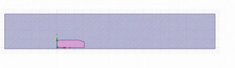
sectional view of the enclosure with the Ahmed body
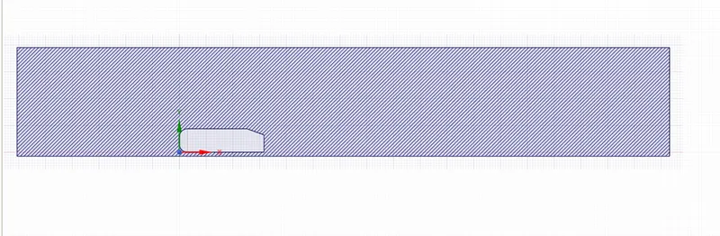
sectional view of the enclosure after hiding and suppressing the body
As the domain and the enclosure are symmetrical along the XY plane, the domain can be divided into half by split body feature along XY plane, which helps us in running the simulation faster with better mesh refinement.
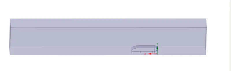
3D view of the divided domain
step-2 Meshing :
Meshing is basically the process of generating a grid i.e, dividing complex geometries into elements that can be used to discretize a domain. First, a baseline mesh is generated(i.e, without changing any parameters) to check the solver settings. If the flow physics works fine, then the mesh refinement is done.
A baseline mesh is generated with 42665 elements and 8597 nodes. The automated mesh is a tetra mesh.
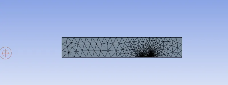
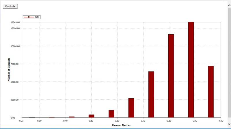
Then the quality of this mesh is checked in the mesh settings, which shows that most of the elements fall under 0.90(1 being the perfect tet-4 shaped element). So, we can proceed further with this base mesh.
Before setting up the solver in Ansys fluent, the boundaries have to be named, by selecting a particular face and naming it.
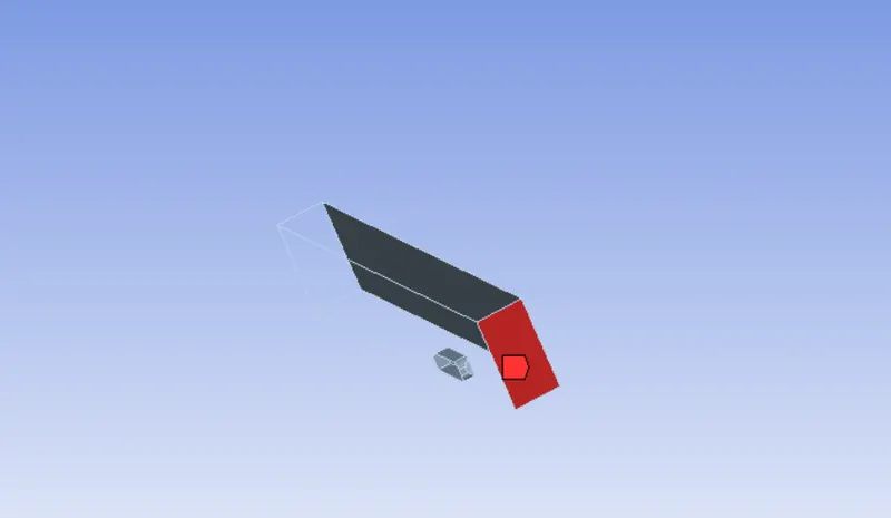
Inlet
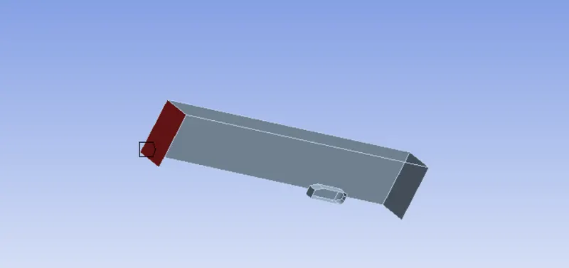
outlet

symmetry
The remaining 4 faces except the inlet and outlet are together named as symmetry.
Before naming the car wall, the faces which interfere from selecting the car wall are to be hidden, and then using the box select, the car walls are selected and named wall.
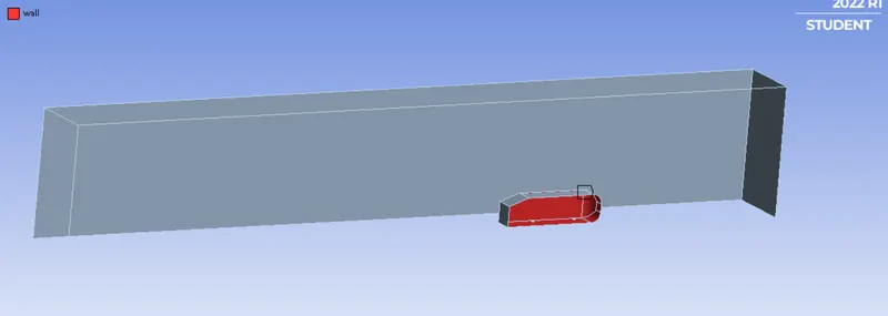
car wall
Now, we can proceed further to set up the physics in Ansys fluent.
Step-3 setting up the solver
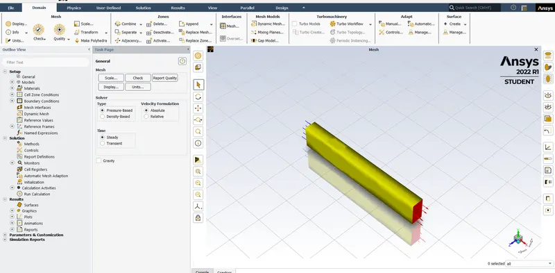
In this step, we define various parameters like initial and boundary conditions, materials used, time steps(for transient), turbulence model, etc which captures the physics to be simulated.
First, we set up the physics by choosing the pressure-based solver as we are dealing with an inlet velocity of 25m/s, which was particularly designed for low-speed incompressible flows(low Mach number), while the density-based solver was mainly designed for high-speed compressible flows(high Mach number).
The steady-state solver is checked, as we are interested to calculate the lift and drag coefficients after the flow variables become steady. The fluid properties are going to be untouched as we are working with default fluid air.
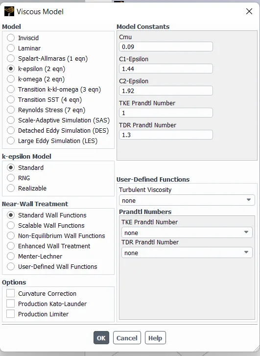
The next parameter that we need to set up is the turbulence model. The turbulence model that we are going to implement is the k-epsilon model.
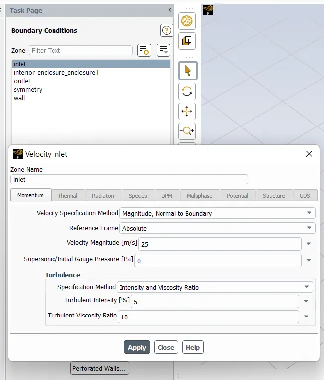
Then the boundary conditions are assigned - inlet velocity-25m/s, outlet - pressure outlet
Hybrid initialization is chosen and works on potential flow theory, which solves the Laplace equation to produce a velocity field that conforms to complex domain geometries, and a pressure field that smoothly connects high and low-pressure values in the computational domain.
After the initialization, reports of lift and drag coefficients are created, and pressure and velocity contours are plotted.
Before creating the lift and drag coefficient plots, the reference values have to be changed, particularly the area, as the coefficients depend on the area exposed to the flow, and other parameters are computed from the inlet.
lift force = 1/2*lift coeff*density*velocity^2*area exposed to the flow
drag force = 1/2*drag coeff*density*velocity^2*area exposed to the flow
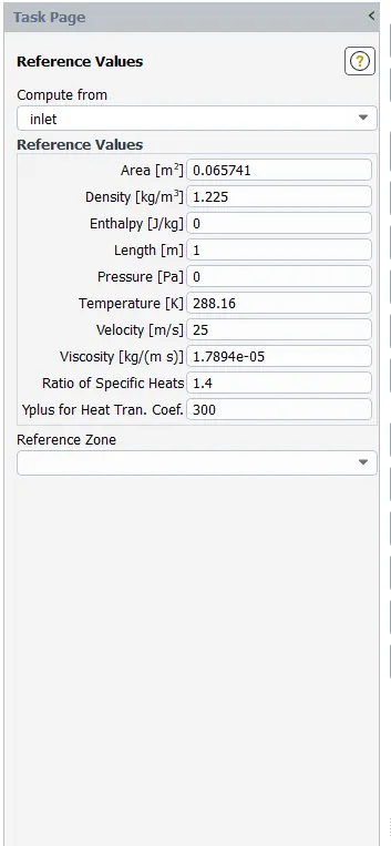
The area exposed to the flow is computed using the projected areas option present in the results.
step-4 solving and Results:
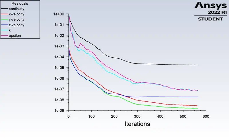
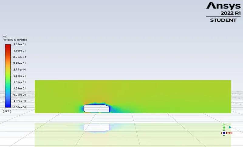
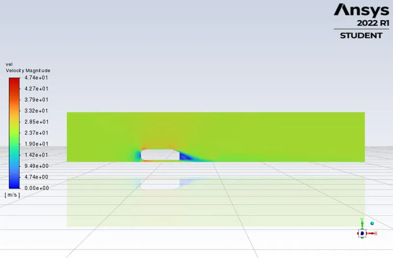
velocity contour
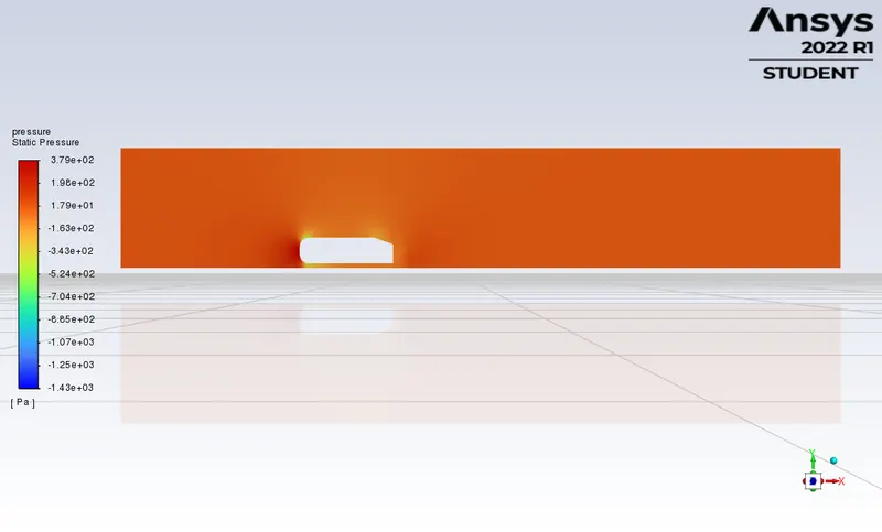
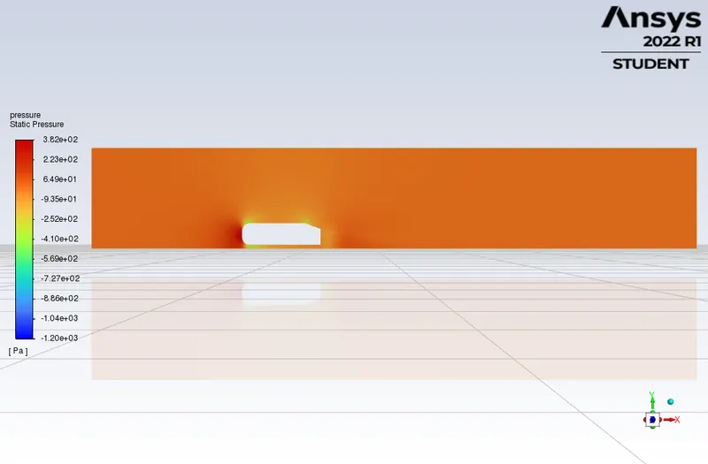
pressure contour
lift coefficient -0.1987487
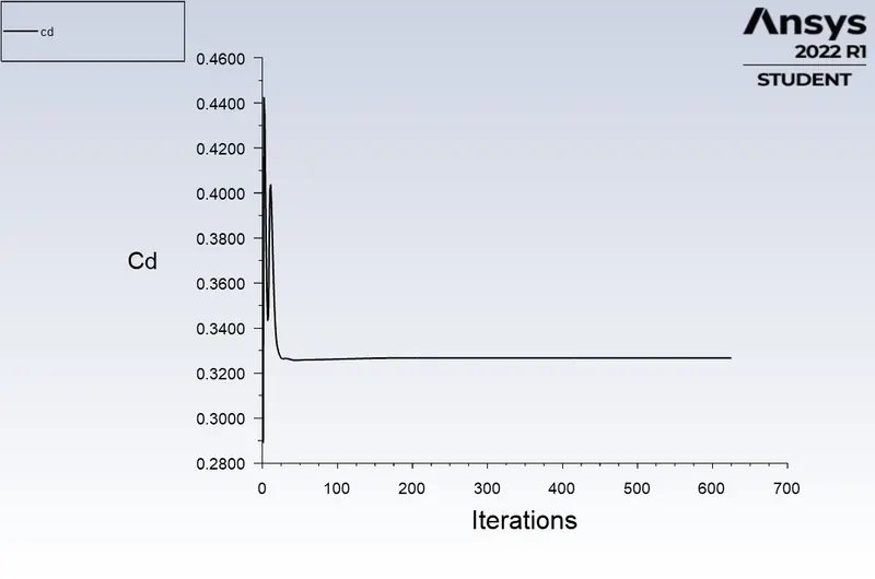
drag coefficient -0.38305379
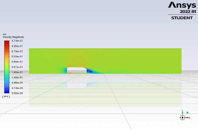
From the above contours, we can say that the wake region was not captured properly due to the coarse mesh(baseline mesh). So, now mesh refinement is being done by creating a local enclosure around the Ahmed body which consists of the wake region. This local enclosure helps a lot, as we can refine the mesh in the local enclosure, not the whole domain, which helps us decrease the cell count and thereby saves the computational power.
Mesh refinement :
First, a local enclosure is created around the Ahmed body in Spaceclaim using the enclosure feature with the below dimensions, which particularly captures the wake region.
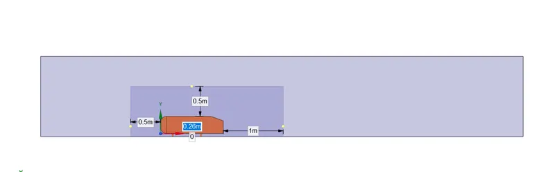
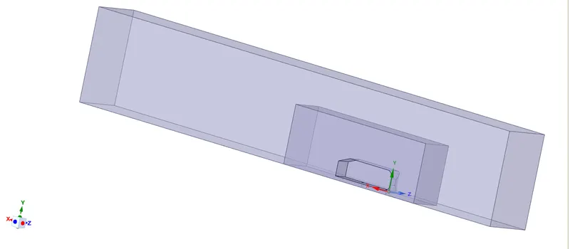
3D view of the domain after creating the local enclosure
But the local enclosure volume interferes with the old enclosure volume.
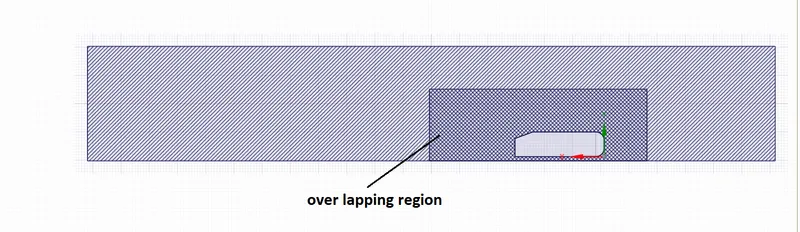
sectional view of the domain
So, the interference feature is used, which automatically detects the overlapping volumes and resolves the problem by subtracting the local enclosure volume from the bigger volume.
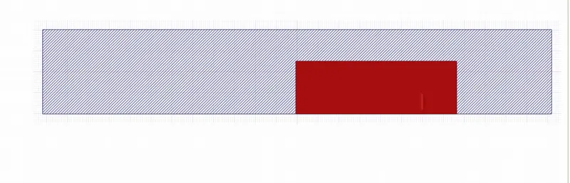
interference detecting the overlapping volumes(red)
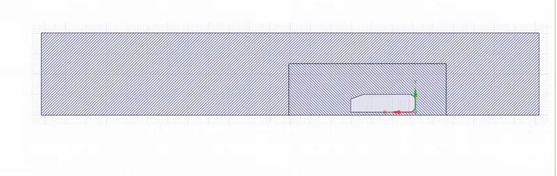
sectional view after using the interference feature
Then, we proceed further to meshing.
Before entering the meshing module, the shared topology should be turned on, which shares information from the bigger volume to the smaller volume.
The idea is that we create a general mesh and apply different meshing strategies to it.
1. The first mesh refinement technique that is applied, is the Multi-zone meshing method, which creates Hexa mesh in the outer region and tetra mesh in the local region.
Mesh --> insert --> Method --> select the outer domain -->Multi zone method --> element size:100mm -->generate mesh.
To get a neat-looking mesh, the maximum element size is made equal to the element size in mesh settings.
2. Then, the inner domain is further refined by using the body sizing method, which helps us capture the physics even more accurately.
Mesh --> insert --> sizing --> select the inner domain --> element size:50mm --> generate mesh .
3. When the bottom face is observed, the rods which support the Ahmed body look like a polygon rather than a circle. So, the rods are refined further to get a circular shape by using the face sizing method
Mesh --> insert --> sizing --> select the faces of the rod --> element size:5mm --> generate mesh .
4. The near-wall modeling significantly impacts the solution, as the walls are the main source where the mean vorticity and turbulence vary. After all, it is in the near-wall region that the solution variables have large gradients, and the momentum and other scalar transports occur most vigorously. Therefore, accurate representation of the flow in the near-wall region becomes of utmost importance.
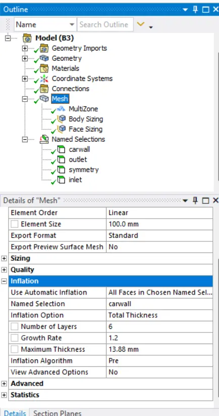
So, inflation layers or body-fitted mesh are created along the car walls.
Mesh settings --> Inflation --> choose the car wall(named selection) --> total thickness --> number of layers:6 --> maximum thickness : 13.88mm --> generate mesh.
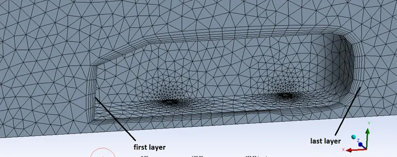
The total thickness of the inflation layers is calculated using the below formulae :

As we are working with the k-epsilon turbulence model( based upon the inbuilt wall functions), to capture the near-wall phenomena the desired y+ ranges from 30 to 300.
Initial desired y+ = 100, characteristic length=1.004m(length of the Ahmed body in the flow direction) the first cell thickness comes out as 1.4mm. Then with a growth rate of 1.2, the total layer thickness is calculated to be 13.88mm.
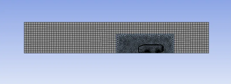
after mesh refinement
The boundary conditions are assigned similar to the baseline setup.
Now, we can proceed further to set up the solver in Ansys fluent, which is the same as the previous settings.
Mesh independency test :
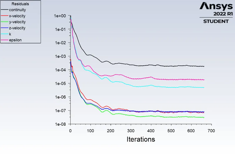
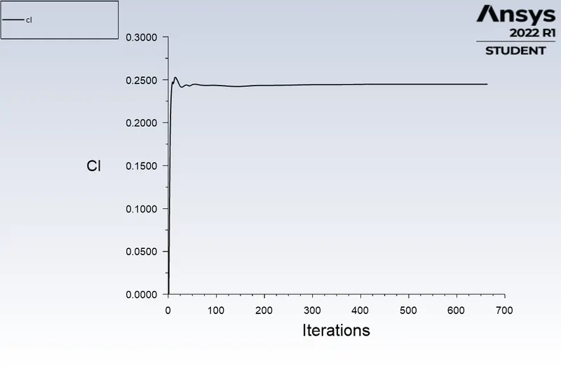
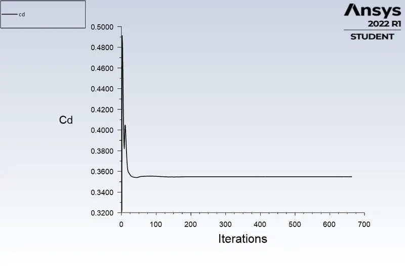
| outer domain(mm) | inner domain(mm) | y+ | first layer thickness(mm) | total thickness(mm) | lift coeff(cl) | drag coeff(cd) | drag error(%) | cell count | node count | |
| case-1 | 100 | 50 | 100 | 1.4 | 13.88 |
0.24472427 |
0.35486437 |
6.06 |
91905 |
31142 |
| case-2 | 75 | 35 | 80 | 1.1 | 11.63 |
0.24850383 |
0.32670212 |
3.03 |
208861 | 61232 |
| case-3 | 60 | 30 | 60 | 0.87 | 8.72 |
0.24055996 |
0.31320422 |
6.06 |
328099 | 96069 |
| case-4 | 60 | 25.2 | 40 | 0.58 | 5.81 |
0.23311289 |
0.29831381 | 12.12 | 503544 | 127715 |
case-1:
lift coefficient plot
drag coefficient plot
velocity contour plot
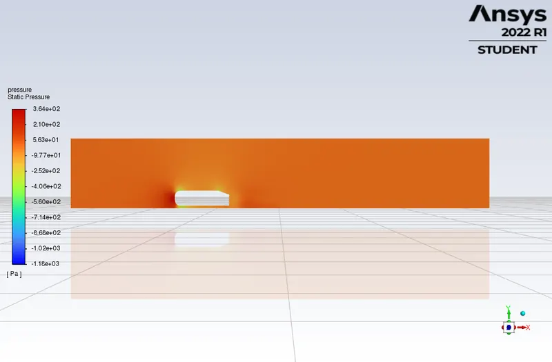
pressure contour plot
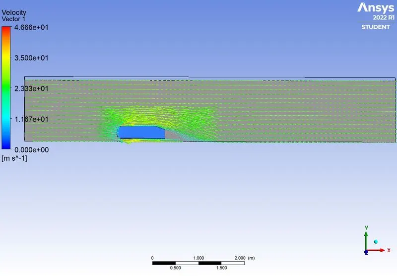
velocity vector plot
case-2:
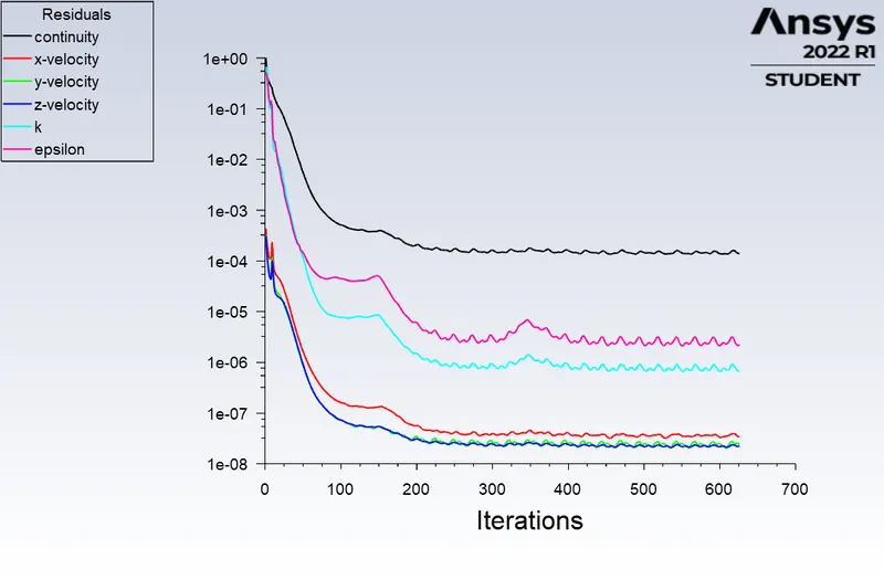
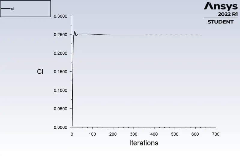
lift coefficient plot
drag coefficient plot
velocity contour plot
pressure contour plot
velocity vector plot
case-3:
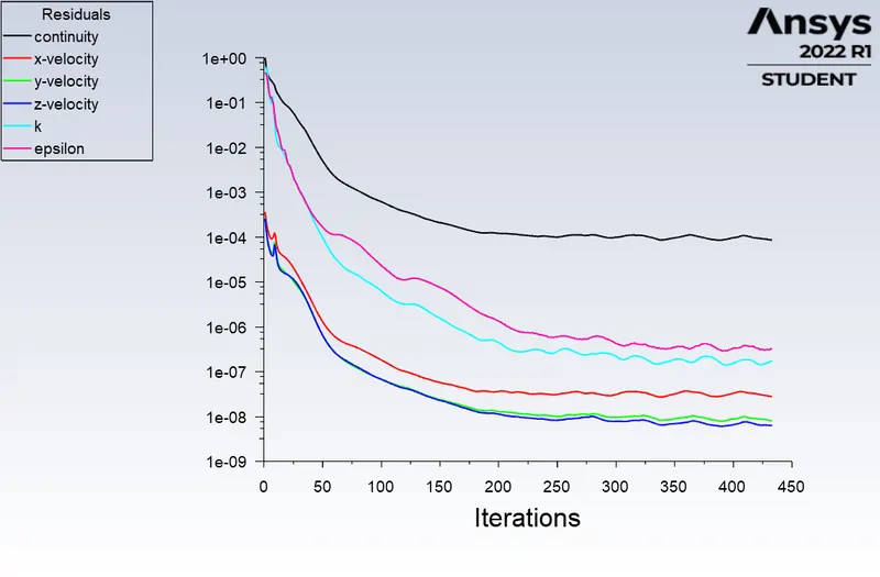
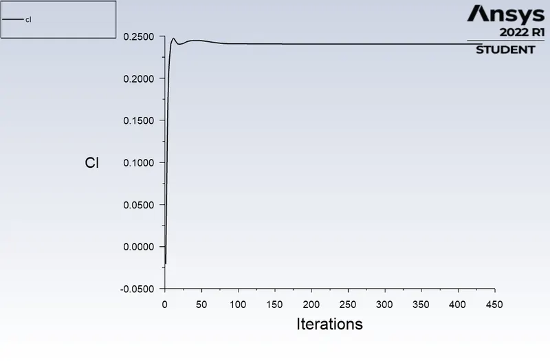
lift coefficient plot
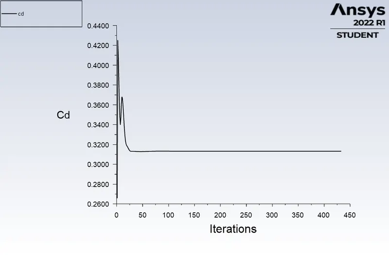
drag coefficient plot
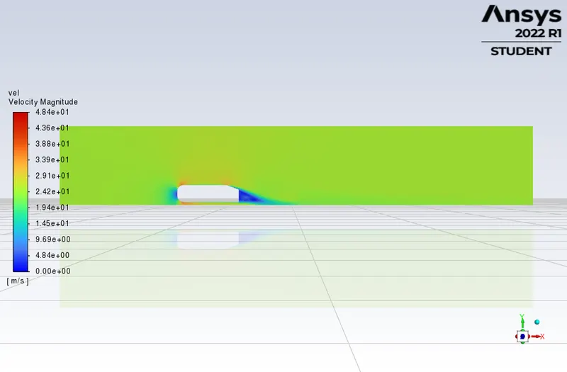
velocity contour plot
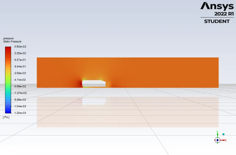
pressure contour plot
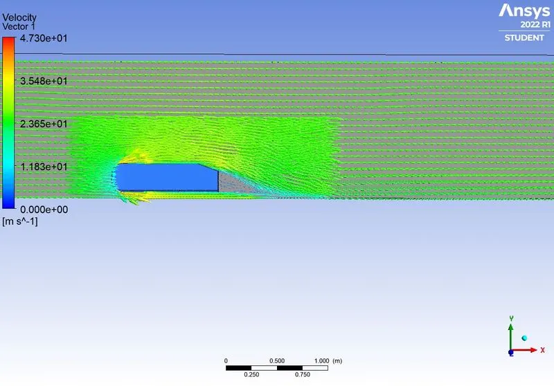
velocity vector plot
case-4:
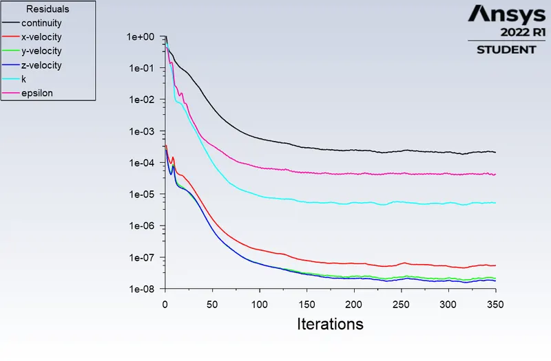
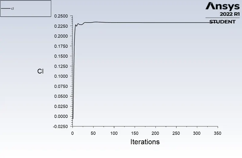
lift coefficient plot
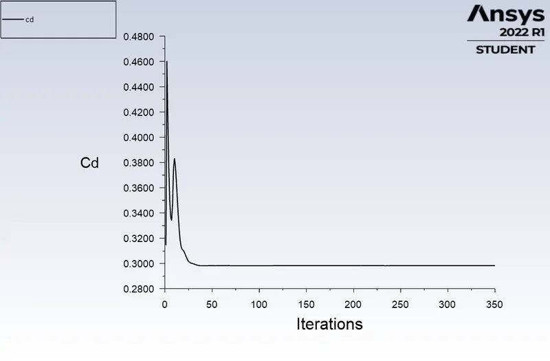
drag coefficient plot
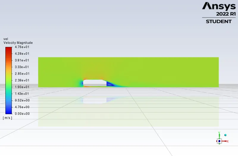
velocity contour plot
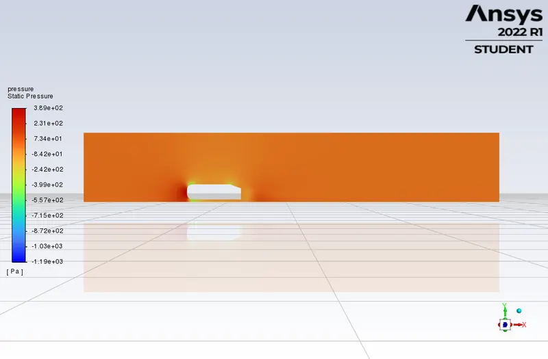
pressure contour plot
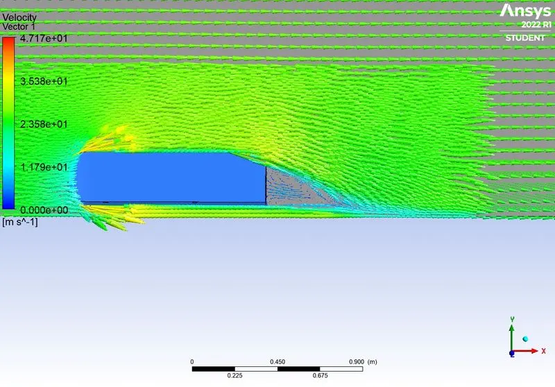
velocity vector plot
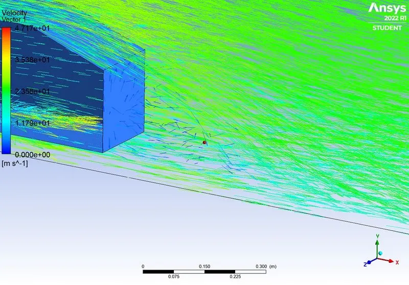
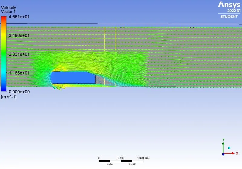
vector plot of velocity in the wake region showing the recirculation zone
Explanation of the physics :
The flow around vehicles is a rather complex phenomenon that includes massive separations and the development of a wake. The boundary layer on the surface of the body eventually separates as it reaches the rear edge and the separated flow experiences high shear and forms a wake. The aerodynamic resistive force that a vehicle experience is mostly due to pressure which means that there is a large pressure difference between the front and the rear of the body. The low-pressure region at the rear is due to the existence of a wake that is made up of multiple lengths and time scales and is inherently unsteady and three-dimensional. These flow features arise due to the bluffness of the geometry and this bluffness is associated with comfort and functionality which cannot be negated.
The Ahmed body was introduced by Ahmed, Fatin, and Ram in 1984, they conducted studies varying the wake topology i.e, rear slant angle, and analyzed its effect on the drag coefficient(cd). The minimum and maximum drag occurred when α ≈ 12.5 º and α ≈ 30.0º, respectively. The increase in drag is attributed to the emergence of the counter-rotating longitudinal vortices called the C-pillar vortices(recirculation zone). These vortices increase the three-dimensionality of the wake which in turn increases the drag. The separation point of the flow greatly influences the wake topology as well as the drag experienced by the body. The lower drag coefficient is associated with separation at the
top slant edge since it prevents the C-pillar vortices from developing.
Conclusion :
1. When external flow over the Ahmed Body is simulated, the recirculation zone and separation of boundary layer have been observed and analyzed.
2. In the baseline setup, the wake region could not be clearly captured (coarse mesh ). So, the mesh was refined and inflation layers that capture the near-wall phenomenon accurately were created.
3. By maintaining the y+ value in the appropriate range, the drag error can be decreased. In this case, when y+ was 80, the drag error was found to be minimum(3.03%).