Week 8 - Simulating Cyclone separator with Discrete Phase Modelling

Aim :

1. To perform analysis on cyclone separator and analyze the efficiency by changing the particle size, and flow velocity (particle velocity).

2. To implement the discrete phase model for this application.

Introduction :

Cyclone separators or simply cyclones are separation devices that use the principle of inertia to remove particulate matter from flue gases. Cyclone separators are one of many air pollution control devices known as pre-cleaners since they generally remove larger pieces of particulate matter. This prevents finer filtration methods from having to deal with large, more abrasive particles later on. Cyclones are particularly well suited for high temperature and pressure conditions because of their rugged design and flexible component materials.
Cyclone collection efficiencies can reach 99% for particles bigger than 5 µm and can be operated at very high dust loading.

In a cyclone separator, fluid along with the mixture of particles is fed into a chamber. The inside of the chamber creates a spiral vortex, similar to a tornado. The lighter components of this gas have less inertia, so it is easier for them to be influenced by the vortex and travel up it. Contrarily, larger components of particulate matter have more inertia and are not as easily influenced by the vortex.

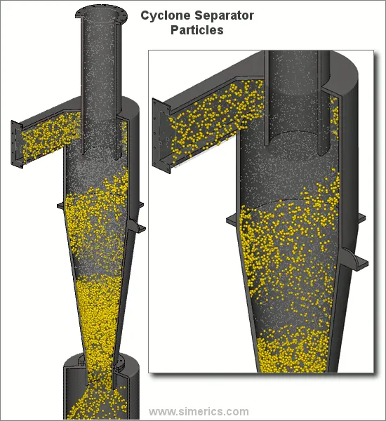
Since these larger particles have difficulty following the high-speed spiral motion of the gas and the vortex, the particles hit the inside walls of the container and drop down into a collection hopper. These chambers are shaped like an upside-down cone to promote the collection of these particles at the bottom of the container. The cleaned flue gas escapes out the top of the chamber.

CYCLONE EFFICIENCY EMPIRICAL MODELS:

1. Iozia and Leith Model:
Iozia and Leith model is a modified version of the Barth Model, which is developed based on force balance. The model assumes that a particle carried by the vortex endures the influence of two forces: a centrifugal force, Z, and flow resistance, W. The collection efficiency ηi of particle diameter dpi can be calculated from

`eta = 1/(1+ (d_(pc) + d_(p i)) ^beta )`

β is an expression for the slope parameter

2. Li and Wang Model :
The Li and Wang model includes particle bounce or re-entrainment and turbulent diffusion at the cyclone wall. A two-dimensional analytical expression of particle distribution in the cyclone is obtained. Li and Wang's model was developed based on the following assumptions:

• The radial particle velocity and the radial concentration profile are not constant for uncollected particles within the cyclone.

• Boundary conditions with the consideration of turbulent diffusion coefficient and particle bounce re-entrainment on the cyclone wall are:
c = c0, at θ = 0

• The tangential velocity is related to the radius of the cyclone by: `mu R^n = constant`

The resultant expression of the collection efficiency for a particle of any size is given as :

`eta_i = 1-exp(-lambda*theta_1)`

3. Koch and Licht Model:

In 1972, Leith and Licht presented another theory (back-mixing) for the study of cyclone collection efficiency. Their back-mixing theory suggests that the turbulent mixing of uncollected particles in any plane perpendicular to the cyclone axis produces a uniform uncollected dust concentration through any horizontal cross-section of a cyclone. Based upon this theory, they developed a model to predict efficiency for any size particles
Koch and Licht collection theory recognized the inherently turbulent nature of cyclones and the distribution of gas residence times within the cyclone. Koch and Licht described particle motion in the entry and collection regions with the additional following assumptions:

• The tangential velocity of a particle is equal to the tangential velocity of the gas flow, i.e. there is no slip in the tangential direction between the particle and the gas.

• The tangential velocity is related to the radius of the cyclone by `mu R^n = constant`

A force balance and an equation on the particles collection yield the grade efficiency ηi

`eta_i =1- exp{-2[(G tau_iQ)/D^3(n+1)]^((0.5)/(n+1))}`

4. Lapple Model:
Lapple model was developed based on force balance without considering the flow resistance. Lapple assumed that a particle entering the cyclone is evenly distributed across the inlet opening. The particle that travels from the inlet half width to the wall in the cyclone is collected with 50% efficiency. The semi-empirical relationship developed by Lapple to calculate a 50% cut diameter, dpc, is

`d_(pc) = [ (9mub)/(2piN_enu_i(rho_p-rho_g))]^(1/2)`

The efficiency of collection of any size of particle is given by

`eta = 1/(1+ (d_(pc) + bard_(p i)) ^2 )`

In any CFD analysis, the workflow that is followed is

Setting up the geometry ----> Meshing ----> setting up the solver ---->solving ---->post-processing results

step-1 Setting up the geometry :

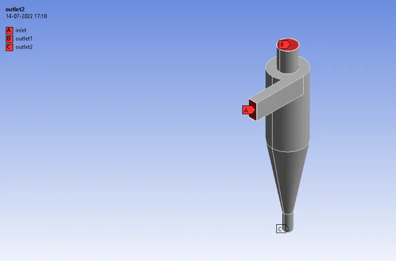
First, we import the pre-modeled cyclone separator geometry into the SpaceClaim module to make changes according to the simulation's requirement. The geometry is a shell geometry i.e, it has a thickness around the flow region. In this CFD analysis, the focus is to track the particles in the flow domain. So, we extract the fluid volume by a feature Volume Extraction and select the inlet and outlet edges i.e, the edges which act as boundaries to the flow domain.

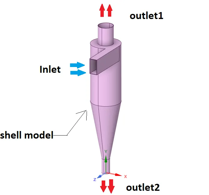
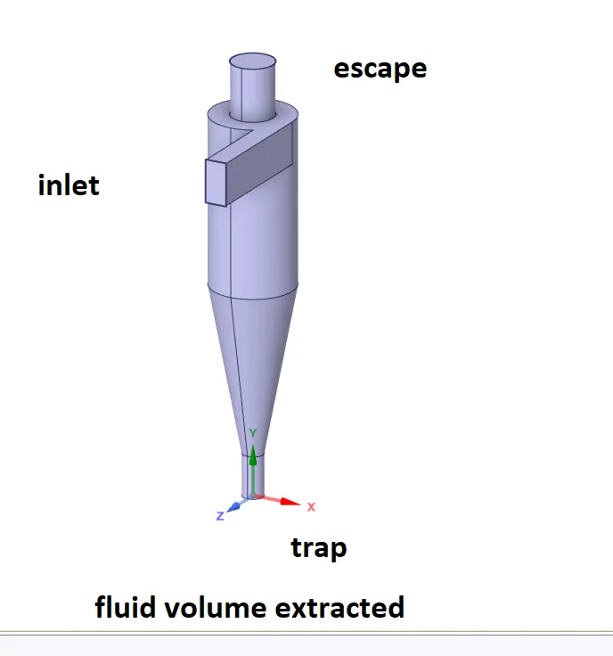
As we are interested only in the flow inside the domain and not about the stresses, strains, etc developing in the geometry. So, the shell/geometry is suppressed for physics.

step-2 Meshing :

Meshing is basically the process of generating a grid i.e, dividing complex geometries into elements that can be used to discretize a domain. A body fitted cartesian mesh is generated which creates a structured mesh of hexahedron elements.

Mesh --> Insert method --> select the body --> body cartesian method --> generate mesh

The element size has been chosen to be 5mm with 425081 elements and 453596 nodes, as it creates an adequate number of particles at the inlet face.

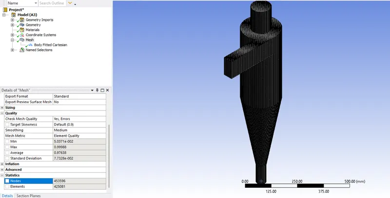
Then the appropriate faces are selected and named accordingly.

step-3 Setting up the solver in Ansys FLuent:

In this step, we define various parameters like initial and boundary conditions, materials used, time steps(for transient), turbulence model, etc which captures the physics to be simulated.

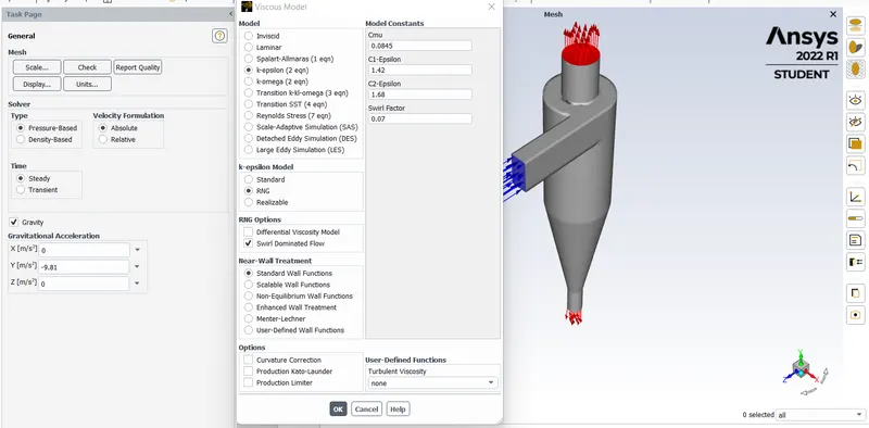
First, we set up the physics by choosing the pressure-based solver which was particularly designed for low-speed incompressible flows(low Mach number), while the density-based solver was mainly designed for high-speed compressible flows(high Mach number). As the cyclone separator works on the principle of inertia, the gravity field is enabled to act in the negative y-direction. Then, the steady-state solver is checked, as we are interested in seeing the final results after the flow variables become steady.

The next parameter that needs to be set up is the turbulence model. For this case, RNG k-epsilon model with swirl-dominated flow is selected.

The focus of this analysis is to track the particles that are going to be injected through the inlet face. To create particles entering along with the fluid discrete phase model is used.

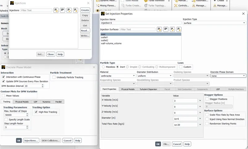
The lagrangian discrete phase model in ANSYS Fluent follows the Euler-Lagrange approach. The fluid phase is treated as a continuum by solving the Navier-Stokes equations, while the dispersed phase is solved by tracking a large number of particles, bubbles, etc through the calculated flow field. The discrete phase can exchange momentum, mass, and energy with the fluid phase.

Under the discrete phase model, interaction with the continuous phase is turned on. And then under injections, the injection type is selected as a surface injection through the inlet face. The particle type is selected as inert and the material as anthracite. Then the velocity of 3m/s is given to the particle in the normal direction i.e, along the x-axis.

Then the boundary conditions are given as follows:

inlet velocity - 3m/s DPM boundary type- reflect

outlet1(top outlet) - pressure outlet DPM boundary type - escape

outlet2(bottom outlet) - pressure outlet DPM boundary type - trap

wall - stationary wall DPM boundary type -reflect

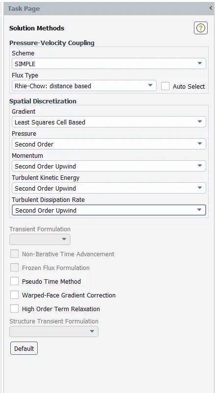
The solution method is changed to a SIMPLE scheme and second-order schemes are adopted for all the variables.

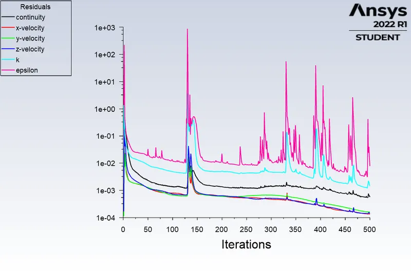
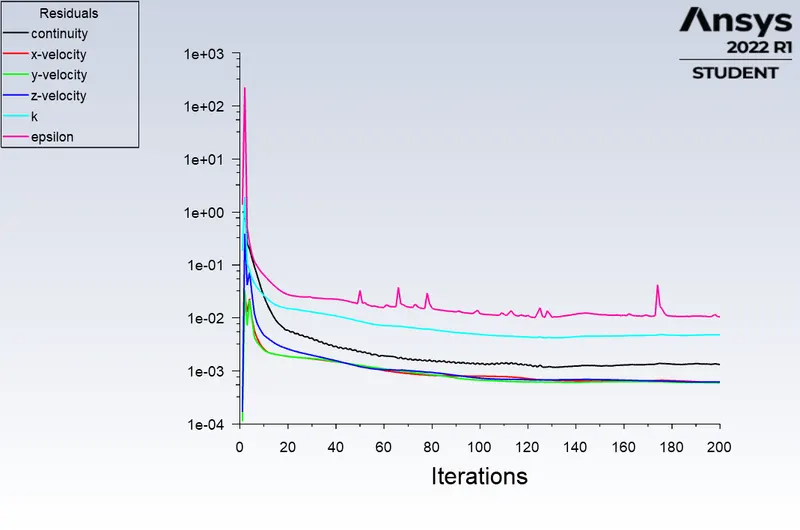
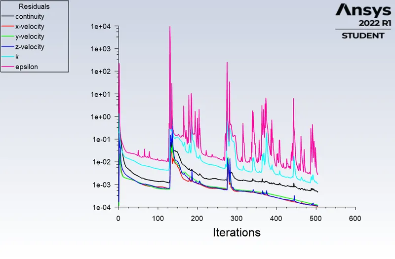
Then solution initialization is done using standard initialization and the flow variables are computed from the inlet. After the initialization, the solver is run.

Step-4 Results :

To analyze the effect of particle size on the cyclone efficiency :

case-1 : particle diameter size = 1micrometer, particle velocity=3m/s

particle tracking animation :

number tracked = 378, escaped = 84, trapped = 294

case-2 : particle diameter size = 3micrometer , particle velocity = 3m/s

particle tracking animation :

number tracked = 378, escaped = 97, trapped = 281

case-3 : particle diameter size=5micrometer , particle velocity = 3m/s

particle tracking animation :

number tracked = 378, escaped = 91, trapped = 293

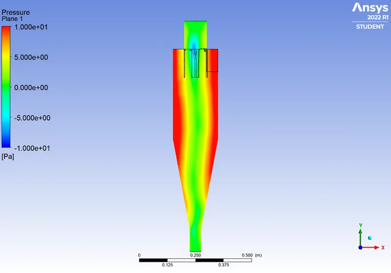
pressure contour:

To analyze the effect of particle flow velocity on the cyclone efficiency :

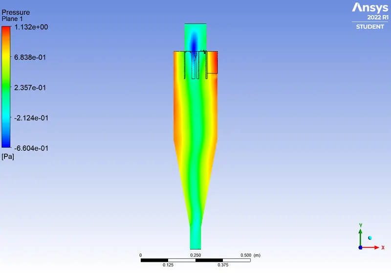
case-4 : particle diameter size=5micrometer , particle velocity = 1m/s

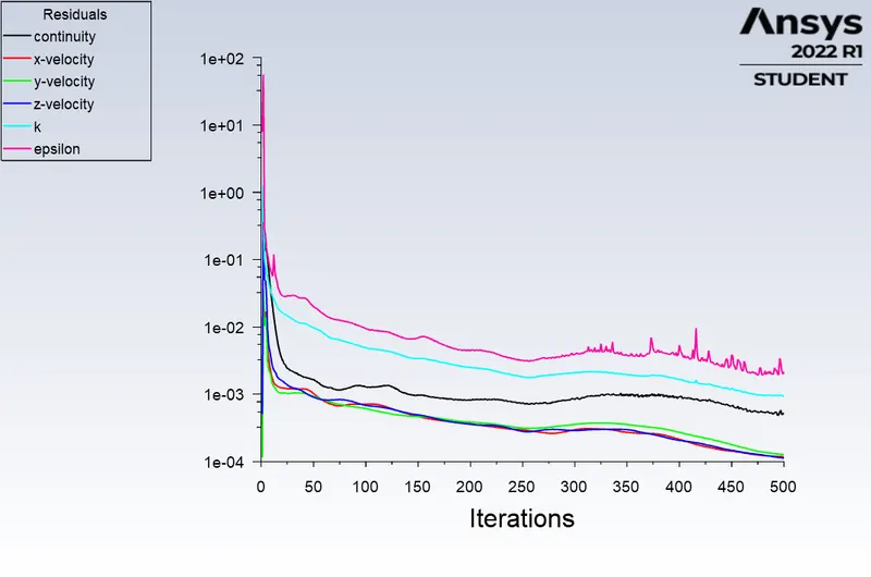
particle tracking animation :

number tracked = 378, escaped = 145, trapped = 233

pressure contour :

case-5 : particle diameter size=5micrometer , particle velocity = 4m/s

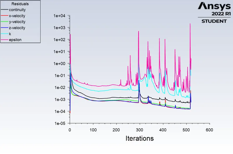
particle tracking animation :

number tracked = 378, escaped = 172, trapped = 206

pressure contour:

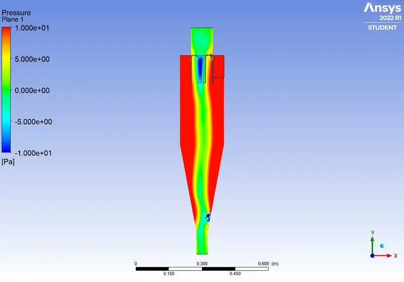
case-6 : particle diameter size=5micrometer , particle velocity = 5m/s

particle tracking animation :

number tracked = 378, escaped = 190, trapped = 188

pressure contour:

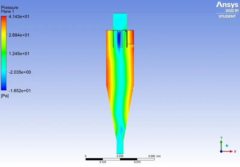
Explanation of the pressure contour:

The pressure contour shows that the static pressure decreases radially from wall to center, and a negative pressure zone appears in the center. The pressure gradient is the largest along the radial direction, as there is a highly intensified forced vortex. the primary flow pattern consists of an outer spiral moving downward from the cyclone inlet and an inner spiral of a smaller radius moving upward into the exit pipe (known as outer vortex and inner vortex).

Observation and Conclusion:

Effect of particle size:

Sno	particle size(micrometer)	Number of particles tracked	number of particles escaped from top outlet	number of particles trapped in the bottom outlet	cyclone efficiency(particles trapped/particles tracked)
case1	1 micrometer	378	84	294	0.777
case2	3 micrometer	378	69	309	0.817
case3	5 micrometer	378	85	293	0.775

As the particle size increases, the cyclone efficiency increases.

Effect of inlet velocity :

Sno	particle size	inlet velocity	number of particles tracked number	number of particles escaped from top outlet	number of particles trapped in the bottom outlet	cyclone efficiency	pressure drop=inlet pressure-outlet pressures
case3	5micrometer	1m/s	378	145	233	0.62	1.390
case1	5micrometer	3m/s	378	85	293	0.775	15.799
case4	5 micrometer	4m/s	378	172	206	0.554	30.567
case5	5 micrometer	5m/s	378	190	188	0.497	48.250

As the inlet velocity increases, the pressure drop increases, and the cyclone efficiency decreases.