Week 5.1 - Mid term project - Solving the steady and unsteady 2D heat conduction problem
Aim :
To solve the 2D heat conduction equation for both steady-state and unsteady-state using iterative solvers using the Jacobi method, gauss seidel method, and successive over-relaxation method for both implicit and explicit schemes
Theory :
case 1: steady-state analysis, implicit method.
The 2D heat conduction equation for steady-state is given by :
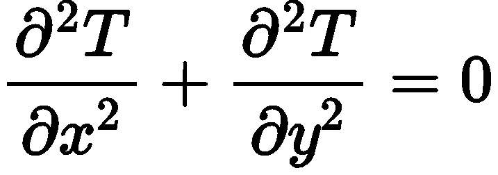
Discretizing the above equation using the central differencing scheme
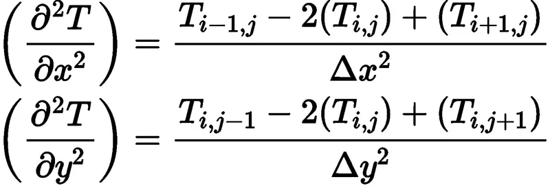
Adding both of the above terms and rearranging we get :

k=2*(dx^2+dy^2)/dx^2+dy^2
dx=element size along x-axis
dy=element size along y-axis
Matlab Code :
% solving 2D heat conduction steady state equation
%d^2 t/d x^2 + d^2 t / d y^2 =0

clear all
close all
clc

%inputs
%length of the domain
l_x=1;
l_y=1;
nx=10; %dividing the domain into elements/nodes
ny=10;
x=linspace(0,l_x,nx); % creating the nodes across the domain
y=linspace(0,l_y,ny);
dx=x(2)-x(1);         % distance between two nodes/length of an element
dy=y(2)-y(1);
k=2*(dx^2+dy^2)/(dx^2*dy^2);


%solving for the temperature values across the rectangular domain in the second iteration by applying discretised DE of heat conduction using the initial values of temperature

%initializing array
t=300*ones(nx,ny);

% assigning boundary conditions
t_t=600;
t_b=900;
t_l=400;
t_r=800;


t(1,2:nx-1)=t_t;
t(ny,2:nx-1)=t_b;
t(2:ny-1,1)=t_l;
t(2:ny-1,nx)=t_r;

%calculating the average temp at corners
t(1,1)=(t_t+t_l)/2;
t(1,nx)=(t_t+t_r)/2;
t(1,ny)=(t_l+t_b)/2;
t(nx,ny)=(t_b+t_r)/2;

%Assigning initial values to t
told=t;
t_initial=t;

%solving the 2D heat conduction equation
%t(i,j)=1/k*[[t(i-1,j)+t(i+1,j)]/dx^2] + [[t(i,j+1)+t(i,j-1)]/dy^2]
error=9e9;
tol=1e-4;
iterative_solver=2;

if iterative_solver==1;
    jacobi_iter=1;

    while(error>tol)

        for i=2:nx-1
            for j=2:ny-1

                term1=(told(i-1,j)+told(i+1,j))/(dx^2*k);
                term2=(told(i,j+1)+told(i,j-1))/(dy^2*k);

                t(i,j)=term1+term2;

            end
        end
        error=max(max(abs(told-t)));
        told=t;
        jacobi_iter=jacobi_iter+1;
    end
    %plotting
    figure(1)

    [c,h]=contourf(x,y,t,10)
    clabel(c,h)
    colorbar
    colormap("jet")
    set(gca,'ydir','reverse')
    xlabel('X-axis')
    ylabel('Y-axis')
    title(sprintf('number of jacobi iterations =%d',jacobi_iter));

end


if iterative_solver==2
    gs_iter=1;
    while(error>tol)

        for i=2:nx-1
            for j=2:ny-1

                term1=(t(i-1,j)+told(i+1,j))/(dx^2*k);
                term2=(told(i,j+1)+t(i,j-1))/(dy^2*k);

                t(i,j)=term1+term2;


            end
        end
        error=max(max(abs(told-t)));
        told=t;
        gs_iter=gs_iter+1;


    end
    %plotting
    figure(2)

    [c,h]=contourf(x,y,t,10)
    clabel(c,h)
    colorbar
    colormap("jet")
    set(gca,'ydir','reverse')
    xlabel('X-axis')
    ylabel('Y-axis')
    title(sprintf('number of gauss siedel iterations =%d',gs_iter));


end


if iterative_solver==3
    sor_iter=1;
    omega=1.2;
    while(error>tol)

        for i=2:nx-1
            for j=2:ny-1


                term1=(t(i-1,j)+told(i+1,j))/(dx^2*k);
                term2=(told(i,j+1)+t(i,j-1))/(dy^2*k);
                term3=(1-omega)*told(i,j);

                t(i,j)=omega*(term1+term2)+term3;


            end
        end
        error=max(max(abs(told-t)));
        told=t;
        sor_iter=sor_iter+1;


    end
    %plotting
    figure(3)

    [c,h]=contourf(x,y,t,10)
    clabel(c,h)
    colorbar
    colormap("jet")
    set(gca,'ydir','reverse')
    xlabel('X-axis')
    ylabel('Y-axis')
    title(sprintf('number of successive over relaxation iterations =%d',sor_iter));


end
Explanation of the code:
1. First, the domain is created by dividing the length along x and y directions into equal (10) numbers of nodes and calculating dx and dy.
2. Then initial conditions (the whole domain is assumed to have a value of 300) and boundary conditions are defined.
3. The boundary conditions at the corners of the square domain are calculated by averaging the data from both of the edges which share the corner.
for example, while calculating the boundary condition at the left top corner, the temperature values from the left boundary and top boundary are considered and averaged.
4. Then the initial temperature field is assigned as told(told forms the previous iteration values for the current iteration values which are going to be calculated.
5.'if' loop is used to direct to different iterative methods.
If iterative_solver ==1 then the Jacobi method is going to be implemented.
If iterative_solver ==2 then the gauss seidel method is going to be implemented.
If iterative_solver ==3 then the successive over-relaxation method is going to be implemented.
6. Two 'for' loops are used to compute the temperature values along x and y directions using the data from the initial conditions, the loop counter variables(i,j) start from the 2nd node and move up to the second last node(nx-1/ny-1) [as the first and last nodes are defined as boundary conditions].
7. Then the error term is computed as the max(max(abs(told - t))) which is the maximum of the absolute value between the current iteration and the previous iteration(i,e, the residual).
8. The error value is computed to check that the temperature values are converged/have become stable(i.e, the difference between the previous and current iterated values is very less, in this case, 1e-4). So, a 'while loop is used with the condition that the error should be greater than the tolerance value.
9. Initially, for the while loop to be executed, the error is assumed to be 9e9, but after every iteration, the error value gets updated till it falls below the tolerance value(1e-4).
10. And after every iteration the t values are stored in told ( i.e, the current iterated values act as old/previous iterated values for the next iteration).
11. For the Jacobi method, the left, right, top, and bottom values are taken from the initial temperature field. Whereas in the Gauss Siedel method, the surrounding values that are already computed are taken and those that are not yet computed are taken from the initial temperature domain. The successive over-relaxation method uses either the Jacobi method or the gauss seidel method as the base.
12. 'contourf' cmd is used to plot the temperature field across the xy domain.
'clabel' cmd labels the contour plot.
'colorbar' cmd displays a vertical color bar to represent different colors for different ranges.
'colormap(jet)' cmd maps the contour to a predefined colormap as a three-column array with the same number of rows as the colormap.
14. To get a proper contour of the temperature field, the y-direction has to be reversed. So, 'set' cmd is used.
15. The title of the plot is given as the number of iterations it took to converge for a particular iterative method.
Plots:
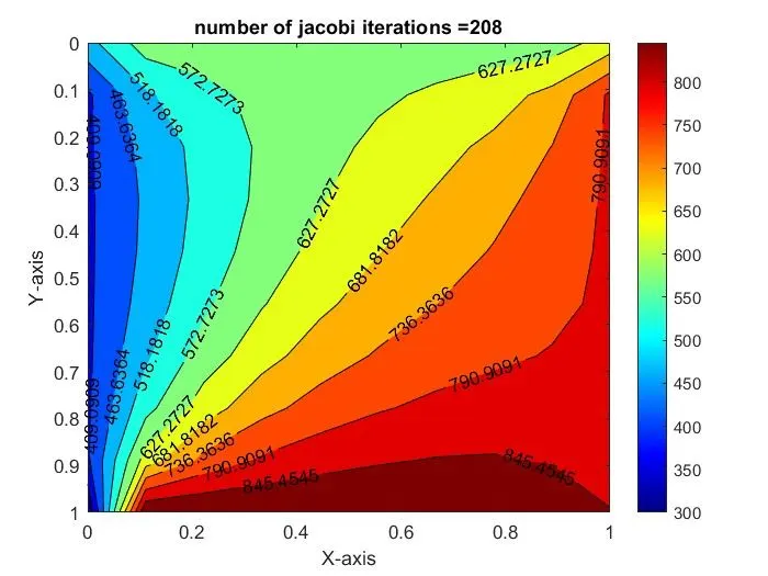
Jacobi method
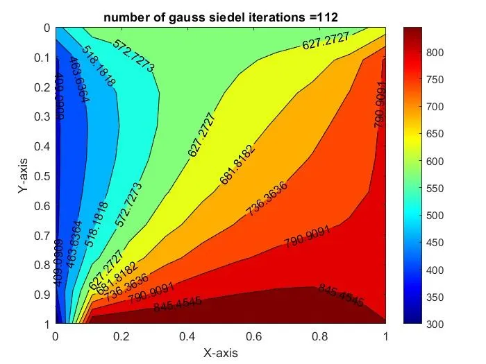
gauss seidel method
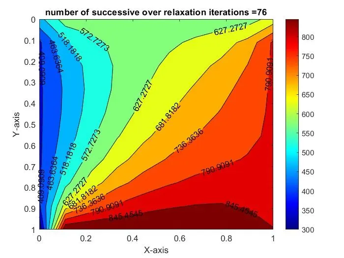
successive over-relaxation method
Conclusion:
| S.no | Iterative method | Number of iterations |
| 1 | Jacobi method | 208 |
| 2 | Gauss Siedel method | 112 |
| 3 | Successive over-relaxation method | 76 |
1. In steady-state analysis, the successive over-relaxation method proves to be more effective compared to the Jacobi and gauss Siedel methods (effectiveness: SOR>GS>Jacobi).
2. The number of iterations in the SOR method depends upon the relaxation factor(omega).
when omega=0, the number of iterations taken for the solution to converge will be the same as that of the Jacobi/Gauss-Seidel method.
As omega approaches 1 from the left limit(below 1), the number of iterations for the solution to converge decreases.
when omega>1, the number of iterations for the solution to converge will decrease up to a certain value of omega(approx 1.5), then the number of iterations increases, and then the solution blows up.
case-2: transient state analysis, explicit method.
The transient state 2D heat conduction is given by :
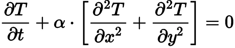
Discretizing the above equation using a forward differencing scheme for time derivatives and a central differencing scheme for space derivatives :

where k1=alpha*dt/dx^2
k2=alpha*dt/dy^2
In the case of the explicit method, the data to compute the temperature field is solely taken from the previous time step.
Matlab code:
% solving transient state 2d heat conduction equation(explicit method)
clear all
close all
clc

%inputs
%length of the domain
l_x=1;
l_y=1;
nx=10; %dividing the domain into elements/nodes
ny=10;
x=linspace(0,l_x,nx); % creating the nodes across the domain
y=linspace(0,l_y,ny);
dx=x(2)-x(1);         % distance between two nodes/length of an element
dy=y(2)-y(1);
dt=1e-3;

%initializing array
t=300*ones(nx,ny);

% assigning boundary conditions
t_t=600;
t_b=900;
t_l=400;
t_r=800;


t(1,2:nx-1)=t_t;
t(ny,2:nx-1)=t_b;
t(2:ny-1,1)=t_l;
t(2:ny-1,nx)=t_r;

%calculating the average temp at corners
t(1,1)=(t_t+t_l)/2;
t(1,nx)=(t_t+t_r)/2;
t(1,ny)=(t_l+t_b)/2;
t(nx,ny)=(t_b+t_r)/2;

%Assigning initial values to t
told=t;
t_initial=t;
alpha=1.1;


k1=alpha*(dt/dx^2);
k2=alpha*(dt/dy^2);
nt=1400;
error=9e9;
tol=1e-4;


%solving the discretized eqn


iter=1;

    for l=1:nt
         error=9e9;
        while(error>tol)

            for i=2:nx-1
                for j=2:ny-1
                    term1=told(i,j);
                    term2=k1*(told(i+1,j)-2*told(i,j)+told(i-1,j));
                    term3=k2*(told(i,j+1)-2*told(i,j)+told(i,j-1));
                    t(i,j)=term1+term2+term3;

                end
            end
            error=max(max(abs(t-told)));
            told=t;
            iter=iter+1;


        end


    end


%plotting
figure(1)
[c,h]=contourf(x,y,t,10);
clabel(c,h);
colorbar;
colormap("jet");
set(gca,'ydir','reverse');
xlabel('X-axis');
ylabel('Y-axis');
title(sprintf('number of iterations(explicit) =%d',iter));
Explanation of the code:
1. The same above explanation implies to this code as well. As this is a transient state analysis, an extra 'for' loop is used for computing the temperature field at each time step.
2. The information required to compute the temperature field is solely taken from the previous time step.
3. And after the computation of the temperature field at a particular time step, it is assigned as told(as it acts as the previous time step for the next time step which is yet to be calculated).
4. The error value needs to be updated after each time step. So, the error term is placed in the time loop.
Contour Plot:
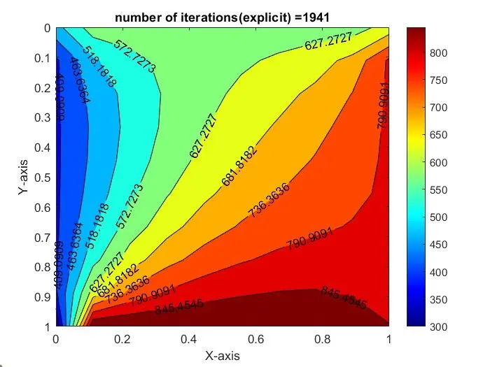
explicit method
case-3: transient-state analysis, implicit method.
The transient state 2D heat conduction is given by :
Discretizing the above equation using a forward differencing scheme for time derivatives and a central differencing scheme for space derivatives :

| |
| |
V V
previous time step current time step
where k1=alpha*dt/dx^2
k2=alpha*dt/dy^2
in the case of the implicit method, the surrounding(left, right, top, bottom) data is taken from the current time step as well as from the previous time step.
Matlab code:
% solving transient state 2d heat conduction equation(explicit method)
clear vars
close all
clc

%inputs
%length of the domain
l_x=1;
l_y=1;
nx=10; %dividing the domain into elements/nodes
ny=10;
x=linspace(0,l_x,nx); % creating the nodes across the domain
y=linspace(0,l_y,ny);
dx=x(2)-x(1);         % distance between two nodes/length of an element
dy=y(2)-y(1);
dt=1e-3;

%initializing array
t=300*ones(nx,ny);

% assigning boundary conditions
t_t=600;
t_b=900;
t_l=400;
t_r=800;


t(1,2:nx-1)=t_t;
t(ny,2:nx-1)=t_b;
t(2:ny-1,1)=t_l;
t(2:ny-1,nx)=t_r;

%calculating the average temp at corners
t(1,1)=(t_t+t_l)/2;
t(1,nx)=(t_t+t_r)/2;
t(1,ny)=(t_l+t_b)/2;
t(nx,ny)=(t_b+t_r)/2;

%Assigning initial values to t
told=t;
t_initial=t;
alpha=1.1;


k1=alpha*(dt/dx^2);
k2=alpha*(dt/dy^2);
nt=1400;
error=9e9;
tol=1e-4;
iterative_solver=2;


if iterative_solver==1;
timestep=1;
jacobi_iter=1;
for l=1:nt
error=9e9;
while(error>tol)
for i=2:nx-1
    for j=2:ny-1

        term1=(1+2*k1+2*k2)^-1;
        H=k1*(told(i+1,j)+told(i-1,j));
        V=k2*(told(i,j-1)+told(i,j+1));
        term2=term1*H;
        term3=term1*V;

        t(i,j)=term1*(t_initial(i,j))+term2+term3;
    end
end
error=max(max(abs(told-t)));
told=t;
jacobi_iter=jacobi_iter+1;

end
t_initial=t;
timestep=timestep+1;


end
figure(1)
[c,h]=contourf(x,y,t,10);
clabel(c,h);
colorbar;
colormap("jet");
set(gca,'ydir','reverse');
xlabel('X-axis');
ylabel('Y-axis');
title(sprintf('number of jacobi iterations(implicit) =%d',jacobi_iter));
end


if iterative_solver==2;
timestep=1;
gs_iter=1;
for l=1:nt
error=9e9;
while(error>tol)
for i=2:nx-1
    for j=2:ny-1

        term1=(1+2*k1+2*k2)^-1;
        H=k1*(told(i+1,j)+t(i-1,j));
        V=k2*(t(i,j-1)+told(i,j+1));
        term2=term1*H;
        term3=term1*V;

        t(i,j)=term1*(t_initial(i,j))+term2+term3;
    end
end
error=max(max(abs(told-t)));
told=t;
gs_iter=gs_iter+1;


end
t_initial=t;
timestep=timestep+1;


end
figure(1)
[c,h]=contourf(x,y,t,10);
clabel(c,h);
colorbar;
colormap("jet");
set(gca,'ydir','reverse');
xlabel('X-axis');
ylabel('Y-axis');
title(sprintf('number of gs iterations(implicit) =%d',gs_iter));
end


if iterative_solver==3;
timestep=1;
omega=1.1;
sor_iter=1;
for l=1:nt
error=9e9;
while(error>tol)
for i=2:nx-1
    for j=2:ny-1

        term1=(1+2*k1+2*k2)^-1;
        H=k1*(told(i+1,j)+t(i-1,j));
        V=k2*(t(i,j-1)+told(i,j+1));
        term2=term1*H;
        term3=term1*V;
        t_gs=term1*(t_initial(i,j))+term2+term3;
        t(i,j)=(1-omega)*told(i,j)+omega*(t_gs);
    end
end
error=max(max(abs(told-t)));
told=t;
sor_iter=sor_iter+1;


end
t_initial=t;
timestep=timestep+1;


end
figure(1)
[c,h]=contourf(x,y,t,10);
clabel(c,h);
colorbar;
colormap("jet");
set(gca,'ydir','reverse');
xlabel('X-axis');
ylabel('Y-axis');
title(sprintf('number of sor iterations(implicit) =%d',sor_iter));
end
Explanation of the code:
1.The same above explanation implies to this code as well.
2.As this is an implicit scheme, the surrounding data is taken from the current time step (previous iteration) as well as from the previous time step(the term t_initial comes into the picture due to the forward differencing scheme of the time derivative). The term t_initial is updated as t after each time step(as this becomes the previous time step for the current time step)
3. The error value needs to be updated after each time step. So, the error term is placed in the time loop.
Contour Plots:
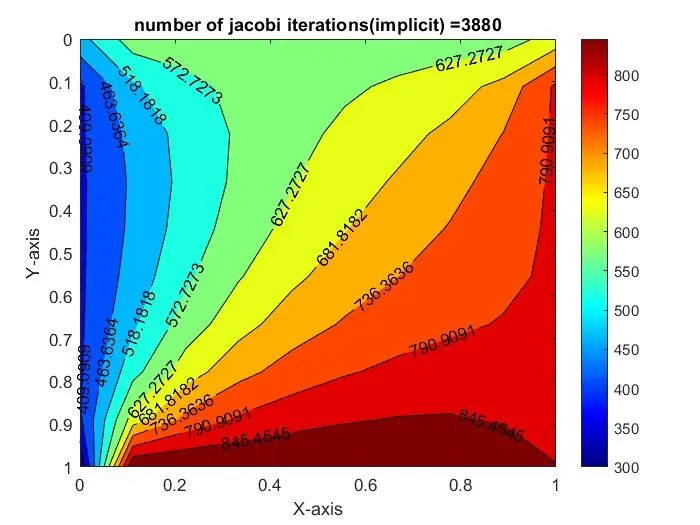
Jacobi method
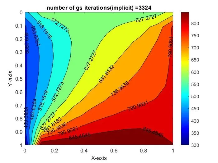
Gauss Siedel method
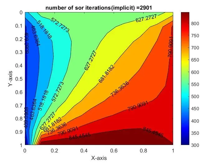
Successive over-relaxation method
Conclusion:
| S.no | Iterative Method | Number of iterations |
| 1 | Jacobi method | 3880 |
| 2 | Gauss Siedel method | 3324 |
| 3 | Successive over-relaxation method | 2901 |
| 4 | explicit method | 1941 |
1. The transient solver requires more number of iterations for the solution to converge compared to the steady-state solver.
2. In transient state analysis, the Successive over-relaxation method proves to be effective compared to Gauss Siedel and Jacobi methods(effectiveness - SOR>GS>Jacobi).
3. The number of iterations in the SOR method depends upon the relaxation factor(omega).
when omega=0, the number of iterations taken for the solution to converge will be the same as that of the Jacobi/Gauss-Seidel method.
As omega approaches 1 from the left limit(below 1), the number of iterations for the solution to converge decreases.
when omega>1, the number of iterations for the solution to converge will decrease up to a certain value of omega(1.1), and then the number of iterations increases, and then the solution blows up.