Week 6 - Understanding the stability analysis in linear systems

Aim:

To see the effect of eigenvalues and spectral radius on the convergence rate while solving the linear system of equations using different iterative methods like Jacobi, Gauss Siedel, and Successive over-relaxation methods.

Matlab code:

Main code:

clear all
close all
clc

% solving the lineaar system of equations ax=b

b=[10; -14; 33];
dold=[5 0 0;0 9 0;0 0 -7];
l=[0 0 0;-3 0 0;1 2 0];
u=[0 1 2;0 0 4;0 0 0];
a=l+u+dold;

%initial guess values
x1=0;x2=0;x3=0;
x=[x1;x2;x3];
xold=x;
error=9e9;
tol=1e-4;
method=1;
dm=linspace(0.1,2,10);



if method==1;
    %jacobi method
    for q=1:length(dm)
        d=dm(q)*dold;

        [x(:,q),jac_iter(q),rho_jac(q),e(:,q)] =jacobi(l,u,d,b);



    end
    subplot(2,1,1)
    plot(dm,jac_iter,LineWidth=2);
    xlabel('magnification factor');
    ylabel('number of jacobi iterations');
    title("Jacobi method","FontSize",15);
    subplot(2,1,2)
    plot(dm,rho_jac,LineWidth=2);
    xlabel('magnification factor');
    ylabel('spectral radius');

end


if method==2;
    % gauss siedel method

    for q=1:length(dm)


        d=dm(q)*dold;

        [x(:,q),gs_iter(q),rho_gs(q),e(:,q)] =gauss(l,u,d,b);



    end
    subplot(2,1,1)
    plot(dm,gs_iter,LineWidth=2);
    xlabel('magnification factor');
    ylabel('number of gs iterations');
    title("Gauss Siedel method","FontSize",15);
    subplot(2,1,2)
    plot(dm,rho_gs,LineWidth=2);
    xlabel('magnification factor');
    ylabel('spectral radius');
end


if method==3;
    % successive over relaxation method
    for q=1:length(dm)


        d=dm(q)*dold;

        [x(:,q),sor_iter(q),rho_sor(q),e(:,q)] =sor(l,u,d,b);


    end
    subplot(2,1,1)
    plot(dm,sor_iter,LineWidth=2);
    xlabel('magnification factor');
    ylabel('number of sor iterations');
    title("Successive over relaxation method","FontSize",15);
    subplot(2,1,2)
    plot(dm,rho_sor,LineWidth=2);
    xlabel('magnification factor');
    ylabel('spectral radius');

end

Explanation of the code :

1. First, the decomposition matrices i.e, the diagonal matrix(d), the lower diagonal matrix(l), and the upper diagonal matrix(d) of the coefficient matrix(A) are defined.

2. Initial guess values for x are assumed and assigned as xold, tolerance(1e-4), magnification factor(dm), and error values are defined.

3. 'if' cmd is used to direct to different iterative methods.

If method==1 then the Jacobi method is implemented.

If method==2 then the gauss seidel method is implemented.

If method==3 then the successive over-relaxation method is implemented.

4. As this challenge focuses on analyzing the effect of diagonal dominance over the convergence rate, the magnification factor array is generated from 0.1 to 2 using linspace cmd.

5. A 'for' loop is used to calculate the x array for different values of magnification factor.

6. The magnification factor is multiplied by the diagonal matrix.

7. To calculate the x array using Jacobi, gauss Siedel, and sor methods, separate functions are created which take the input argument as the diagonal matrix(d), the lower diagonal matrix(l), the upper diagonal matrix(d), and b matrix and return x array, the number of iterations for the solution to reach convergence, eigenvalues and spectral radius.

8. Then to visualize the effect of magnification factor with the number of iterations and spectral radius, graphs are plotted between magnification factor and number of iterations, and between magnification factor and spectral radius.

Function codes :

Jacobi function :

function [x,iter,rho_jac,e] =jacobi(l,u,d,b)

error=9e9;
tol=1e-4;
xold=[0;0;0];
% jacobi method
%solving
iter=1;
while(error>tol)
    x = inv(d)*b-(inv(d)*(l+u))*xold;
    error=max(abs(xold-x));
    xold=x;
    iter=iter+1;

end

%calculating the iteration matrix
tjac=-inv(d)*(l+u);

%calc eigen values
e=roots(poly(tjac));

%calc the spectral radius
rho_jac=max(abs(eig(tjac)));
end

Gauss Siedel function(gauss):

function [x,gs_iter,rho_gs,e]=gauss(l,u,d,b)

error=9e9;
tol=1e-4;
xold=[0;0;0];
% gauss siedel method
%solving
gs_iter=1;
while(error>tol)
    x = inv(l+d)*b-(inv(l+d)*u)*xold;

    error=max(abs(xold-x));
    xold=x;
    gs_iter=gs_iter+1;

end

%calculating the iteration matrix
tgs=-(inv(l+d))*u;

%calc eigen values
e=roots(poly(tgs));

%calc the spectral radius
rho_gs=max(abs(eig(tgs)));
end

Successive over-relaxation(sor)function:

function [x,sor_iter,rho_sor,e]=sor(l,u,d,b)
error=9e9;
tol=1e-4;
xold=[0;0;0];
alpha=0.8;
% sor method
%solving
sor_iter=1;
while(error>tol)
    x = alpha*(inv(l+d)*b)+(1-alpha)*(inv(l+d)*u+ones(3,3))*xold;

    error=max(abs(xold-x));
    xold=x;
    sor_iter=sor_iter+1;
    
end

%calculating the iteration matrix
tsor=ones(3,3)-alpha*(inv(l+d)*u+ones(3,3));

%calc eigen values
e=roots(poly(tsor));

%calc the spectral radius
rho_sor=max(abs(eig(tsor)));
end

explanation of the functions code:

1. The input arguments taken by the above functions are l,u,d,b, and returns x array, spectral radius, the number of iterations, and the eigenvalues.

2. The error, tolerance, and initial guess values are defined.

3. Then the solution/ x array is calculated using the below-mentioned formulae :

a. Jacobi method:

b. Gauss-Siedel method:

c.Successive over-relaxation method:

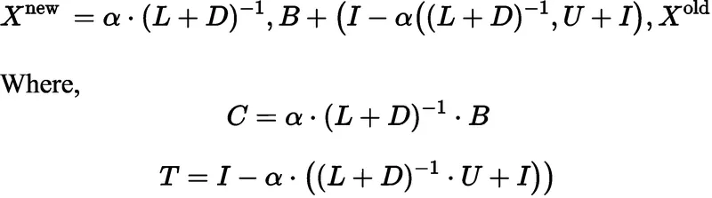
4. After the calculation of current iterated values, it is then assigned as cold (as it acts as the previous iteration for the next iteration which is yet to be calculated).

5. The error term is computed i.e, the maximum absolute difference between the previous iterated matrix and the current iterated matrix. When the error term falls below a tolerance value (i.e, there is a negligible difference between the previous iterated solution array and the current iterated solution array, in this case,1e-4), the solution array is acquired.

6. So, a 'while' loop is used with the condition that the error should be greater than the tolerance value. To enter the while loop initially, the error value is given as 9e9, but after every iteration, the error value gets updated till it falls below 1e-4.

7. Then the iteration/transformation matrix is calculated.

8. The eigenvalues of the iteration matrix are calculated using the 'poly' cmd which forms the characteristic equation of a matrix. Then the roots of the characteristic equation are obtained by 'roots' cmd.

9. The spectral radius of a square matrix is the largest absolute value of its eigenvalues.

Plots:

1.Jacobi method:

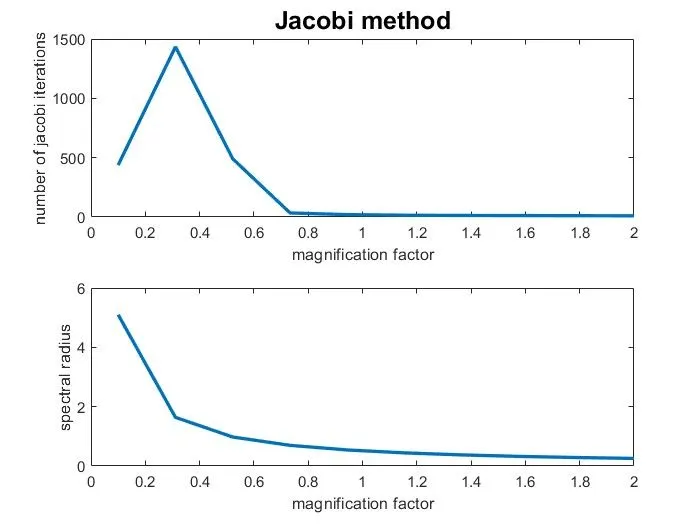
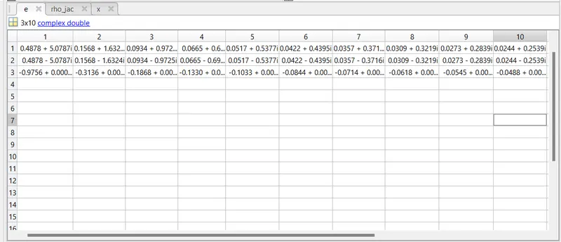
eigenvalues corresponding to different magnification factors

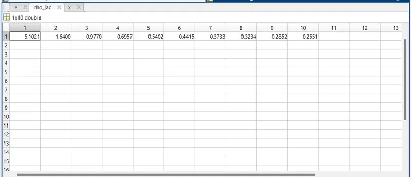
spectral radius corresponding to different magnification factors

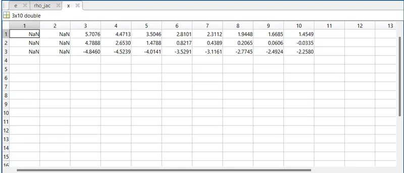
x array corresponding to different magnification factors

number of iterations corresponding to different magnification factors

2. Gauss-Siedel method :

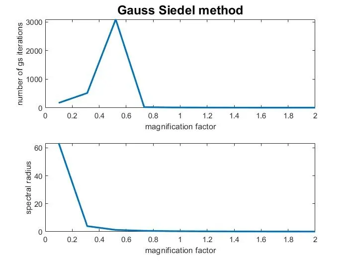
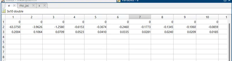
eigenvalues corresponding to different magnification factors

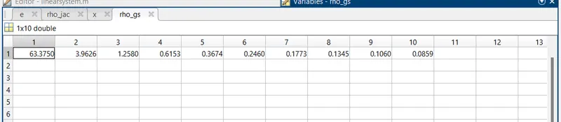
spectral radius corresponding to different magnification factors

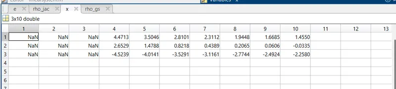
x array corresponding to different magnification factors

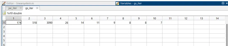
number of iterations corresponding to different magnification factors

3. Successive over-relaxation method:

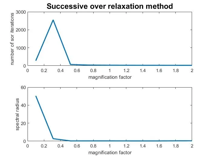
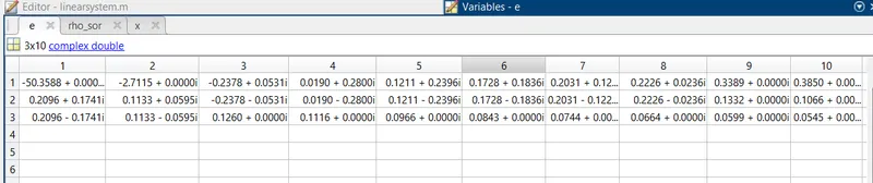
eigenvalues corresponding to different magnification factors

spectral radius corresponding to different magnification factors

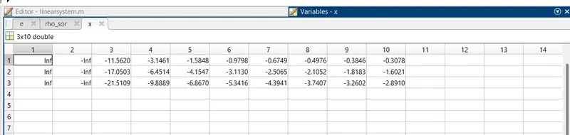
x array corresponding to different magnification factors

number of iterations corresponding to different magnification factors

Conclusion:

1. When the magnification factor is increased, the spectral radius decreases accordingly.

2. The number of iterations for the solution to reach convergence decreases when the magnification factor is increased(spectral radius is decreased).

3. When the spectral radius in any method is greater than 1, then the solution becomes undefined/blows up/unstable.

4. We can finally conclude that when the diagonal dominance increases, the spectral radius decreases, the convergence rate increases, and when the spectral radius falls below 1 the solution becomes stable.