Week 11 - Simulation of Flow through a pipe in OpenFoam
Aim :
1. To simulate the flow through pipe considering an axisymmetric section of the flow by applying the wedge boundary condition.
2. To perform validation studies.
Introduction :
Fluid flow in circular and noncircular pipes is commonly encountered in practice. The hot and cold water that we use in our homes is pumped through pipes. Oil and natural gas are transported hundreds of miles by large pipelines. Blood is carried throughout our bodies by arteries and veins. The fluid flow in pipes is generally driven by the pressure difference.
Consider a fluid entering a circular pipe at a uniform velocity. Because of the no-slip condition, the fluid particles in the layer in contact with the surface of the pipe come to a complete stop. This layer also causes the fluid particles in the adjacent layers to slow down gradually as a result of friction. To make up for this velocity reduction, the velocity of the fluid at the midsection of the pipe has to increase to keep the mass flow rate through the pipe constant. As a result, a velocity gradient develops along the pipe.
The region of the flow in which the effects of the viscous shearing forces caused by fluid viscosity are felt is called the boundary layer. The hypothetical boundary surface divides the flow in a pipe into two regions: the boundary layer region, in which the viscous effects and the velocity changes are significant, and the irrotational(core) flow region, in which the frictional effects are negligible and the velocity remains essentially constant in the radial direction.
The thickness of this boundary layer increases in the flow direction until the boundary layer reaches the pipe center and thus fills the entire pipe. The length from the pipe inlet to the point at which the boundary layer merges at the centerline is called the hydrodynamic entrance length.
hydrodynamic entrance length `L_h=0.06*Re*D`
dynamic viscosity `mu=8.90e-4 N/m^2`
density`rho = 997 (kg)/m^3`
kinematic viscosity`nu=(mu)/rho=(8.90e^-4)/997=8.9267e^-7m/s^2`
velocity profile `u(r)=2V_(avg)(1-r^2/R^2)`
`u(R)=V_(max)=2V_(avg)`
pressure drop`Deltap=p1-p2=(32muLV_(avg))/D^2`
shear stress `tau = - mu (du)/(dr)`
To start a simulation in OpenFOAM, the first step is to choose a tutorial that is similar to a case. The tutorial might not be exactly similar, so, we make necessary changes, might be in the geometry, mesh, solver settings, etc.
In our case, we are interested in simulating the flow through a backward-facing step similar to the 'Cavity' case in the OpenFOAM tutorials. First, we copy the Cavity folder(Incompressible-->icoFoam) from tutorials to the run folder, where the simulations are run. After copying, the first thing that needs to be changed is the geometry and mesh settings in the blockMeshDict file(system->blockMeshDict).
Geometry Modelling:
As the flow is symmetric about the axis, we can solve for a wedge section by considering the below vertices.
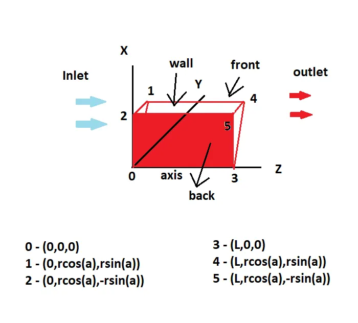
To create the wedge geometry, we require the length of the pipe which depends on the Re number, diameter, and the wedge angle. The parameterization is done in the BlockMeshDict file itself. The vertices are also given in terms of the parameters: length(l), radius(r), and wedge angle.
creating blocks:
In this case, only one box is required.
hex (0 2 1 0 3 5 4 3) ($nx $ny $nz) simpleGrading ($gx $gy $gz)
While defining the box, we orient the box in such a way that the first two vertices(0 2) in the hex represent the direction of the x-axis. Similarly, the second and third vertices(2 1) represent the y-axis, and the first and fifth vertices(0 3) represent the z-axis. This forms the local coordinate system.
Meshing:
The mesh refinement can be changed by changing the values in simple grading cmd. The first value represents the size of the last cell to the size of the first cell in the x-direction. The second and third represent the same in y and z-directions. The number of elements in x,y, and z-directions is represented by the second element, next to simple grading. Even these values are given in terms of parameters.
Boundary Conditions:
Whenever specifying the face notations in the boundary conditions, the order should be in such a way that the notation(cw/ccw) of the points should specify the normal using the right-handed thumb rule. The normal of each and every face should be pointing outwards.
inlet - faces -(0 1 2 0)
outlet - faces - (3 5 4 3)
The inlet and outlet are given patch type bc which indicates that mass transfer can take place.
front - faces - (0 3 4 1)
back - faces - (0 2 5 3)
The front and back faces are given wedge type bc, which is used for axisymmetric geometries.
wall -faces - (2 1 4 5)
axis - faces -(0 3 3 0)
For axis, empty type bc is given, where the calculations are avoided.
editiing the BlockMeshDict file
/*--------------------------------*- C++ -*----------------------------------*\
  =========                 |
  \\      /  F ield         | OpenFOAM: The Open Source CFD Toolbox
   \\    /   O peration     | Website:  https://openfoam.org
    \\  /    A nd           | Version:  9
     \\/     M anipulation  |
\*---------------------------------------------------------------------------*/
FoamFile
{
    format      ascii;
    class       dictionary;
    object      blockMeshDict;
}
// * * * * * * * * * * * * * * * * * * * * * * * * * * * * * * * * * * * * * //

// blockMesh parameterization

/* Geometrical Info */

D	0.004;                      // Diameter
r #calc "0.5*$D";                   // Radius
angle	5;                          // Angle in degrees
theta   #calc "degToRad($angle)";   // Angle in radians
Re 2100;          		    // Reynolds Number
Le #calc "0.06*$Re*$D";             // Entrance Length
L  #calc "0.2 + $Le";		    // Total length of pipe

/* Vertices Info */

xmin	0;
xmax	$L;
ymax	#calc "$r*cos($theta)";
zmax	#calc "$r*sin($theta)";
zmin    #calc "-$r*sin($theta)";

/* Mesh Info */

nx	10;	// Cells along local X
ny	1;	// Cells along local Y
nz	50;	// Cells along local Z
gx	0.2;	// SG along local X
gy	1;	// SG along local Y
gz	1;	// SG along local Z


convertToMeters 1;

vertices
(
    ($xmin 0 0)		 //0
    ($xmin $ymax $zmax)	 //1
    ($xmin $ymax $zmin)	 //2
    ($xmax 0 0)		 //3
    ($xmax $ymax $zmax)	 //4
    ($xmax $ymax $zmin)	 //5

);

blocks
(
    hex (0 2 1 0 3 5 4 3) ($nx $ny $nz) simpleGrading ($gx $gy $gz)
);

edges
(
);

boundary
(
    inlet
    {
        type patch;
        faces
        (
            (0 1 2 0)
        );
    }
    outlet
    {
        type patch;
        faces
        (
            (3 5 4 3)
        );
    }
    front
    {
        type wedge;
        faces
        (
            (0 3 4 1)
        );
    }
    back
    {
        type wedge;    // symmetry
        faces
        (
            (0 2 5 3)
        );
    }
    walls
    {
        type wall;    // symmetry
        faces
        (
            (2 1 4 5)
        );
    }
    axis
    {
        type empty;
        faces
        (
            (0 3 3 0)
        );
    }

);

mergePatchPairs
(
);

// ************************************************************************* //
After changing the vertices, creating blocks, meshing, and assigning the boundary faces in the blockMeshDist file. Paraview is opened, which is a 3D data visualization software, which shows the geometry, the mesh created and also plots the contours of the pressure, velocity, temperature fields, etc at different time steps(based on the solving).
Geometry :
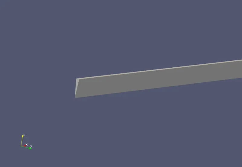
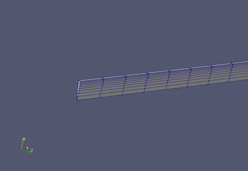
As the initial pressure and velocity fields are defined for the previous geometry. We need to change the faces assigned for different boundaries and the boundary names(according to the case). In the pressure and velocity files, the units are also mentioned, OpenFOAM takes pressure values input as the kinematic pressure i.e, static pressure/density. The initial pressure values at the inner volumes are given as 0 shown by internalField uniform 0. Then to calculate the pressure on the inlet face,the zeroGradient type method, which extrapolates the pressure value from the inner volumes, is used. The outlet pressure value is given as zero gauge pressure. The front and back faces are given wedge type bc.And to calculate the pressure on the walls, zeroGradient type bc is used.The axis is given empty type bc.
Pressure :
/*--------------------------------*- C++ -*----------------------------------*\
  =========                 |
  \\      /  F ield         | OpenFOAM: The Open Source CFD Toolbox
   \\    /   O peration     | Website:  https://openfoam.org
    \\  /    A nd           | Version:  9
     \\/     M anipulation  |
\*---------------------------------------------------------------------------*/
FoamFile
{
    format      ascii;
    class       volScalarField;
    object      p;
}
// * * * * * * * * * * * * * * * * * * * * * * * * * * * * * * * * * * * * * //

dimensions      [0 2 -2 0 0 0 0];

internalField   uniform 0;

boundaryField
{
    inlet
    {
	type            zeroGradient;
    }

    outlet
    {

        type            fixedValue;
        value           uniform 0;
    }

    front
    {
        type            wedge;   // symmetry
    }

    back
    {
        type            wedge;   // symmetry
    }

    walls
    {
        type            zeroGradient;
    }

    axis
    {
        type            empty;
    }
}

// ************************************************************************* //
Similarly, in the velocity file, the faces and the boundary names are changed. Then the values at the inner volumes are given as 0 indicated by internalField uniform(000) (as pressure is a vector). The inlet velocity is calculated based on the flow type i.e, laminar flow(Re=2100)
`Re=(vD)/nu`
where v- inlet velocity to be calculated = 0.46865175m/s
L - characteristic length = diameter of the pipe = 0.004m
nu - kinematic viscosity = 8.9267e^-7m/s^2
The outlet velocity values are calculated using the zeroGradient method.The front and back faces are given wedge type bc.The wall is given noSlip condition and the axis is given empty type bc.
Velocity:
/*--------------------------------*- C++ -*----------------------------------*\
  =========                 |
  \\      /  F ield         | OpenFOAM: The Open Source CFD Toolbox
   \\    /   O peration     | Website:  https://openfoam.org
    \\  /    A nd           | Version:  9
     \\/     M anipulation  |
\*---------------------------------------------------------------------------*/
FoamFile
{
    format      ascii;
    class       volVectorField;
    object      U;
}
// * * * * * * * * * * * * * * * * * * * * * * * * * * * * * * * * * * * * * //

dimensions      [0 1 -1 0 0 0 0];

internalField   uniform (0 0 0);

boundaryField
{
    inlet
    {
        type            fixedValue;
        value           uniform (0.46865175 0 0);
    }

    outlet
    {
        type            zeroGradient;
    }

    front
    {
        type            wedge;   // symmetry
    }

    back
    {
        type            wedge;   // symmetry
    }

    wall
    {
        type            noSlip;
    }

    axis
    {
        type            empty;
    }
}

// ************************************************************************* //
Then the transport Properties which is present in the constant folder are changed.The value of kinematic viscosity is changed to 8.9267e^-7 m^2/s.
Transport properties file:
/*--------------------------------*- C++ -*----------------------------------*\
  =========                 |
  \\      /  F ield         | OpenFOAM: The Open Source CFD Toolbox
   \\    /   O peration     | Website:  https://openfoam.org
    \\  /    A nd           | Version:  9
     \\/     M anipulation  |
\*---------------------------------------------------------------------------*/
FoamFile
{
    format      ascii;
    class       dictionary;
    location    "constant";
    object      transportProperties;
}
// * * * * * * * * * * * * * * * * * * * * * * * * * * * * * * * * * * * * * //

nu              [0 2 -1 0 0 0 0] 8.9267803410231e-07;


// ************************************************************************* //
After changing the parameters which simulate the flow, the simulation run time, time steps, etc are changed in the controlDict file.
controlDict file:
/*--------------------------------*- C++ -*----------------------------------*\
  =========                 |
  \\      /  F ield         | OpenFOAM: The Open Source CFD Toolbox
   \\    /   O peration     | Website:  https://openfoam.org
    \\  /    A nd           | Version:  9
     \\/     M anipulation  |
\*---------------------------------------------------------------------------*/
FoamFile
{
    format      ascii;
    class       dictionary;
    location    "system";
    object      controlDict;
}
// * * * * * * * * * * * * * * * * * * * * * * * * * * * * * * * * * * * * * //

application     icoFoam;

startFrom       startTime;

startTime       0;

stopAt          endTime;

endTime         5;

deltaT          0.001;

writeControl    timeStep;

writeInterval   500;

purgeWrite      0;

writeFormat     ascii;

writePrecision  6;

writeCompression off;

timeFormat      general;

timePrecision   6;

runTimeModifiable true;


// ************************************************************************* //
Post-processing and conclusion :
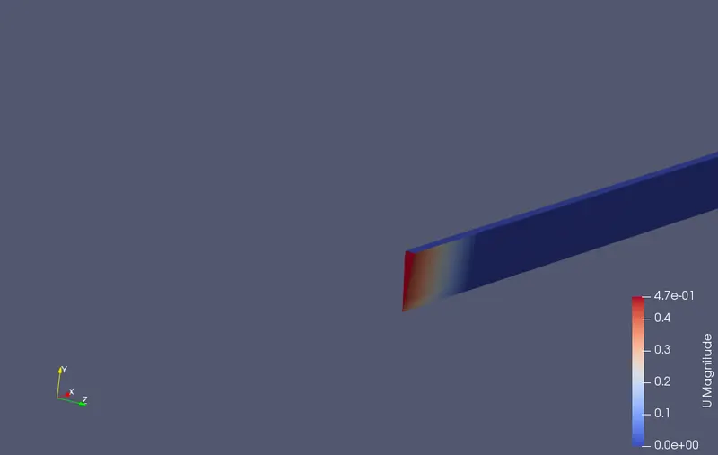
initial velocity contour
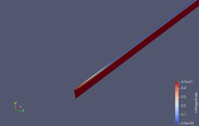
final velocity contour
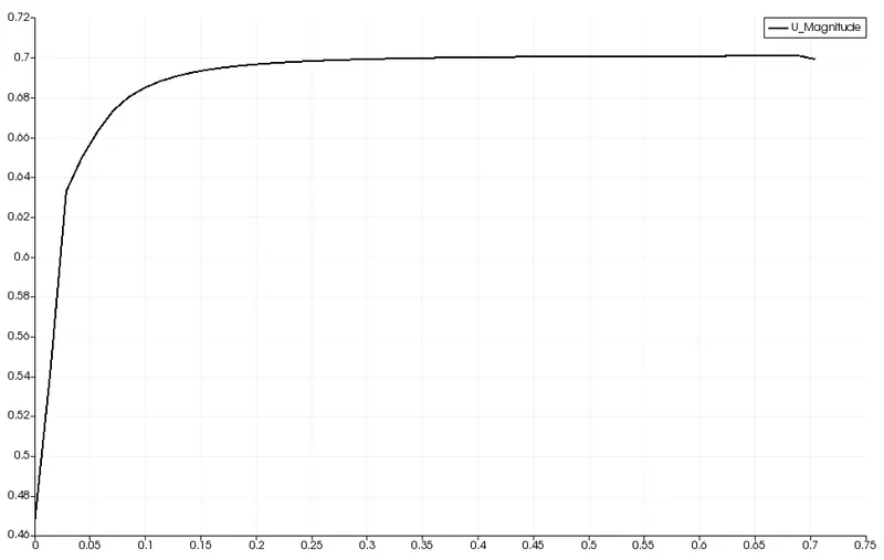
variation of velocity along the length of the pipe
Up to the hydrodynamic length i.e, x=0.504m the velocity varies, and then the velocity becomes almost steady.
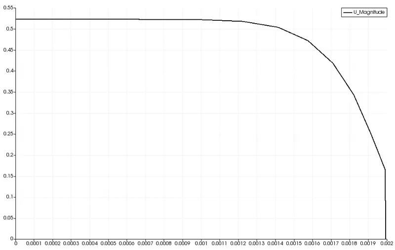
Velocity profile at x=0.01m(inlet)
At the inlet, in the inner core / irrotational regions of the pipe, the velocity profile is constant. But as it approaches the walls, the velocity gradually decreases indicating the formation of a boundary layer due to the no-slip condition(frictional resistance to the flow)
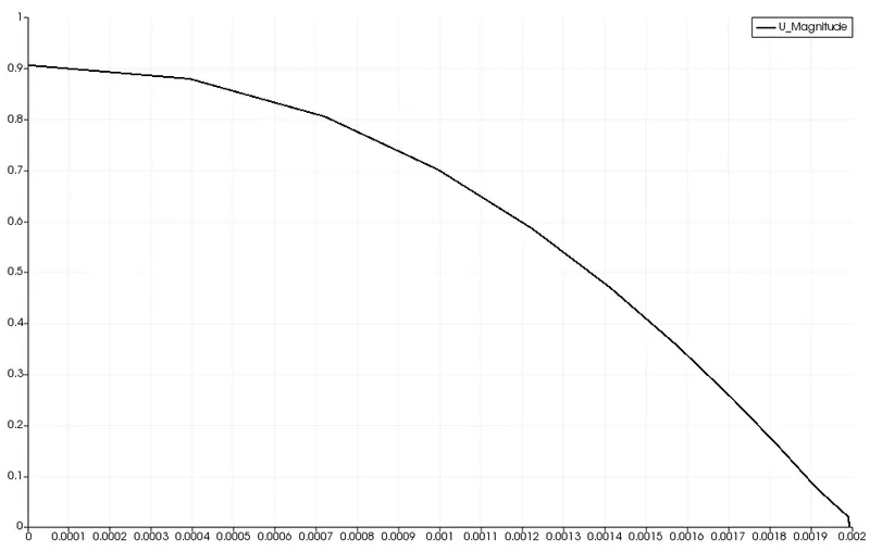
velocity profile at x=0.45m(before Lh)
As the flow progresses, the inner core region decreases, and the boundary layer increases till the pipe center. And then, the boundary layer fills up the entire pipe.
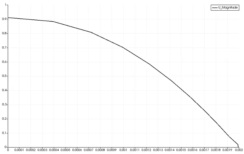
vel profile at x=0.53m
After the flow is fully developed, the velocity profile becomes constant across the length of the pipe.
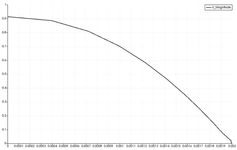
vel profile at x=0.65m
Shear stress is calculated in Paraview using the calculator feature.
`tau=-mu*(du)/(dr)`
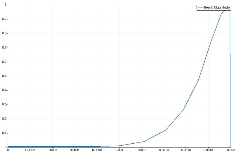
shear stress variation along the arc length at x=0.01m
At the inlet, the shear stress at the wall is greater because the gradient of u near the wall(in radial direction) decreases drastically.
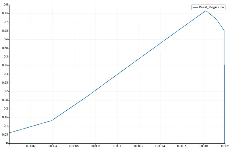
shear stress variation along the arc length at x=0.48m (before Lh)
As the flow progresses, due to the formation of boundary layer, the shear stress near the walls is the highest.
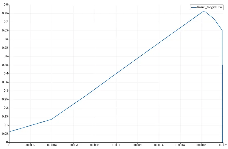
shear stress variation along the arc length at x=0.53m (after Lh)
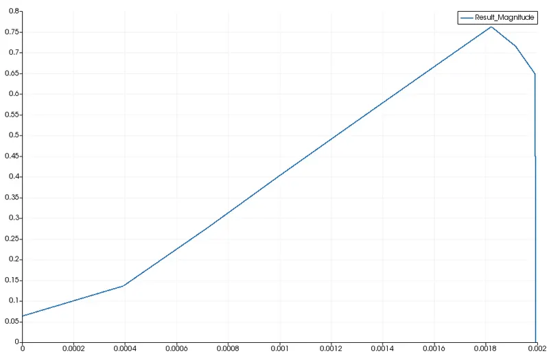
shear stress variation along the arc length at x=0.65m (fully developed flow)
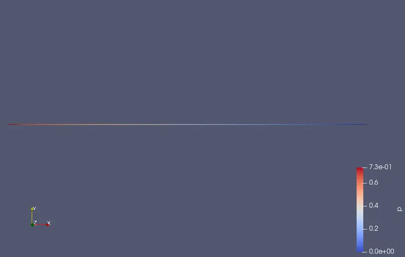
pressure contour
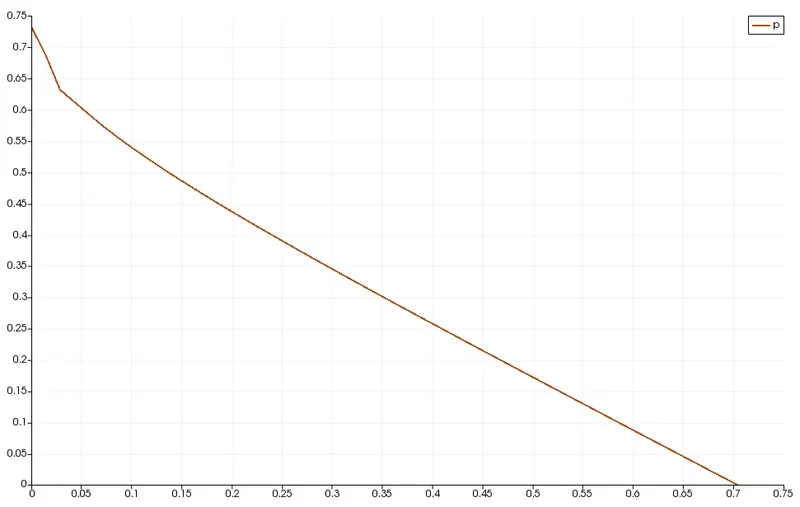
variation of pressure along the x-axis
Validation Study:
Hagen Poiseuille relations:
velocity profile `u(r)=2V_(avg)(1-r^2/R^2)`
`u(R)=V_(max)=2V_(avg)`
pressure drop`Deltap=p1-p2=(32muLV_(avg))/D^2`
shear stress `tau = - mu (du)/(dr)`
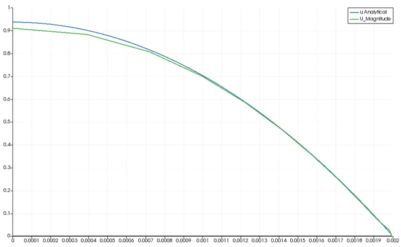
velocity profile validation at x=0.53(fully developed profile)
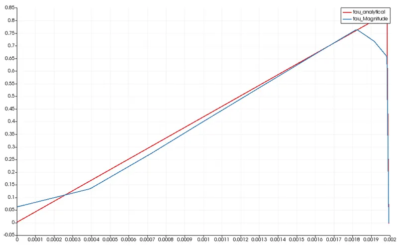
shear stress validation at x=0.53(fully developed flow)
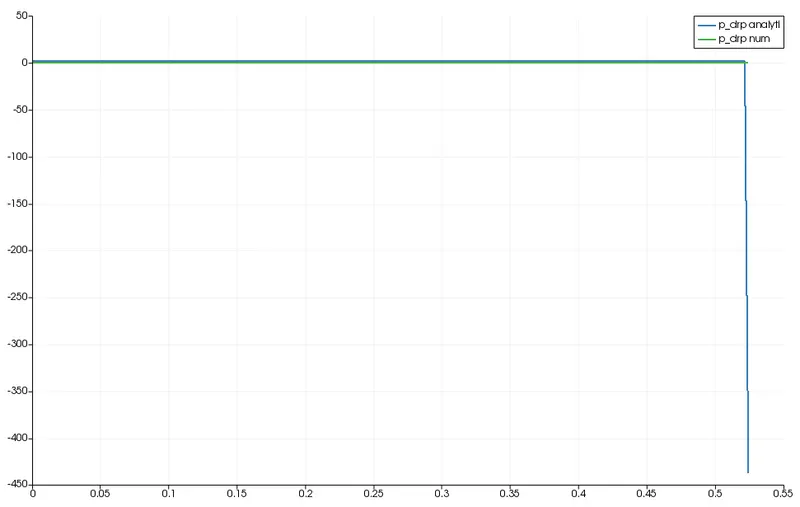
pressure drop validation along the x-axis