Week 5 - Rayleigh Taylor Instability
Aim :
To perform the Rayleigh Taylor instability with various mesh sizes and user-defined fluid to understand the physics behind instabilities and the importance of the Atwood number.
Introduction:
The instability of a heavy fluid layer supported by a light one is generally known as Rayleigh-Taylor (RT) instability. It can occur under gravity and, equivalently, under an acceleration of the fluid system in the direction toward the denser fluid. Because of the transient nature of RT instabilities in common situations, its physical significance may have escaped attention for a long time. Experimental observations of RT instabilities only started with the work of Taylor and Lewis about forty years ago. However, Rayleigh's theoretical analysis dates back to the end of the last century.
Over the past decades, it also became obvious that RT instabilities would play an important role in many different fields. The Rayleigh–Taylor instability has been applied in considering a wide range of problems such as inertial confinement fusion, supernova explosion and remnants, atmospheric physics, geophysics, and oceanography.
The growth of the RTI can be roughly divided into four stages. In the first stage, the amplitude h of the perturbation is much smaller than the wavelength λ. The linear stability theory is valid and shows that the amplitude grows exponentially with time:
h=h0*e^α*t
where h0 is the initial amplitude, α is the growth rate, and t is the time. The growth rate depends on the density ratio (ρH/ρL) or Atwood number At = (ρH − ρL)/(ρH + ρL),[where ρH and ρL are the densities of the heavy and light fluids, respectively], the surface tension, the viscosity, and the compressibility. When the amplitude grows to a size of order 0.1λ to 0.4λ, substantial deviations from the linear theory are observed and the RTI evolves into the second (nonlinear) stage. During the second stage, the light fluid rises into the heavy fluid in the form of bubbles and the heavy fluid falls into the lighter fluid in the form of spikes. In the third stage, the nonlinearity becomes much stronger. The Kelvin–Helmholtz instability occurs due to a velocity difference across the interface between two fluids and a roll-up of vortices forms a mushroom-type shape of the spikes. Also, there is bubble amalgamation, in which large bubbles absorb smaller ones and large bubbles grow larger and move faster. In the final stage, the RTI evolves into a turbulent or chaotic mix
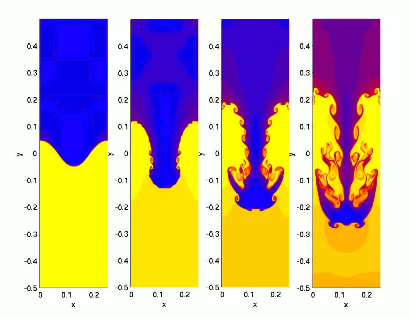
four stages of RT instability
a) sinusoidal interface at base stage b)formation of spikes c)interaction of spikes and bubbles to form larger ones d)turbulent mixing
Some practical CFD models that have been based on the mathematical analysis of Rayleigh Taylor waves :
Richtmeyer-Meshkov instability :
The Richtmyer–Meshkov instability (RMI) occurs when two fluids of different densities are impulsively accelerated. Normally this is by the passage of a shock wave. The development of the instability begins with small amplitude perturbations which initially grow linearly with time. This is followed by a nonlinear regime with bubbles appearing in the case of a light fluid penetrating a heavy fluid, and with spikes appearing in the case of a heavy fluid penetrating a light fluid. A chaotic regime eventually is reached and the two fluids mix. This instability can be considered the impulsive-acceleration limit of the Rayleigh-Taylor instability.
Kevin-Helmholtz instability:
The Kelvin–Helmholtz instability is a fluid instability that occurs when there is velocity shear in a single continuous fluid or a velocity difference across the interface between two fluids. Kelvin-Helmholtz instabilities are visible in the atmospheres of planets and moons, such as in cloud formations on earth or the red spot on Jupiter, and in the atmospheres of the sun and other stars.
In any CFD analysis, the workflow that is followed is
Setting up the geometry ----> Meshing ----> setting up the solver ---->solving ---->post-processing results
step-1 Setting up the geometry :
We want to observe and analyze the fluid instabilities when the denser fluid is on top of the lighter fluid when the gravity field is applied. So, a plane of the 3D experiment would be sufficient. This simple 2D geometry is designed in Spaceclaim using the rectangle and pull features.
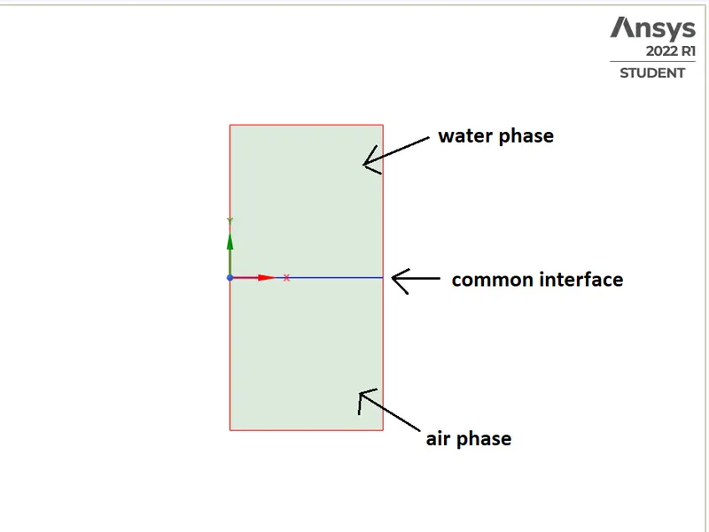
To transfer information between both phases, the common interface should be turned on to share topology using the share feature.
step-2 Meshing :
Meshing is basically the process of generating a grid i.e, dividing complex geometries into elements that can be used to discretize a domain. First, a baseline mesh is generated(i.e, without changing any parameters) to check the solver settings. If the flow physics works fine, then the mesh refinement is done.
First, a base automated (quad dominated)mesh is created with an element size of 0.5mm with 3200 elements and 3321 nodes.
case-1: base mesh element size-0.5mm
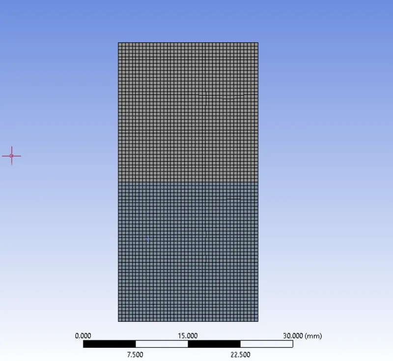
case-2 element size-0.3mm elements - 8978 nodes-9180
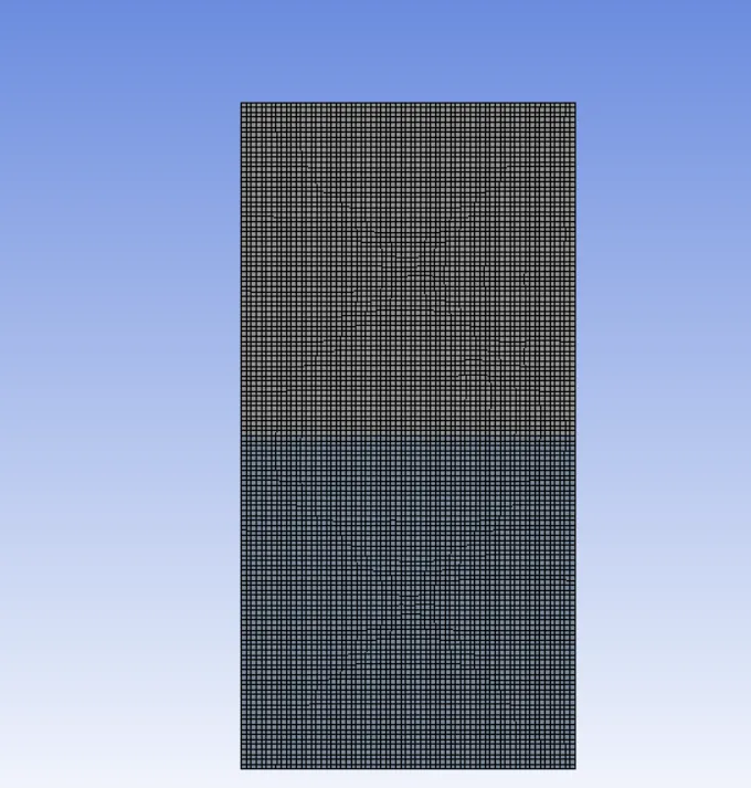
case-3 mesh size=0.1mm elements- 80000 nodes- 80601
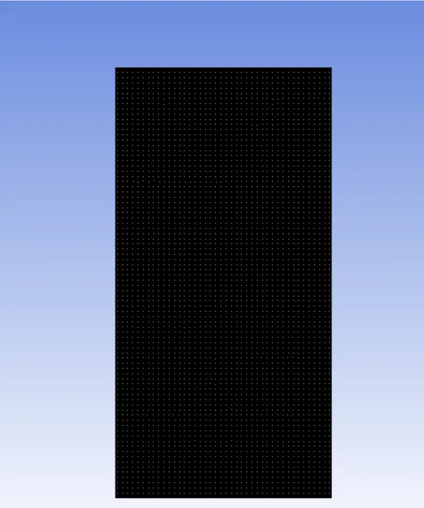
Then the faces are named accordingly, with the water phase as the upper face and the air phase as the lower face.
Now, we can proceed to set up the solver in fluent.
Step-3 setting up the solver
In this step, we define various parameters like initial and boundary conditions, materials used, time steps(for transient), turbulence model, etc which captures the physics to be simulated.
First, we set up the physics by choosing the pressure-based solver as we are dealing with low velocity, which was particularly designed for low-speed incompressible flows(low Mach number), while the density-based solver was mainly designed for high-speed compressible flows(high Mach number). The gravity field is applied in the negative y-direction(-9.81m/s2) as this instability occurs with the application of gravity.
The transient solver is checked. For this approach, transient state analysis is implemented as the physics that evolves, is a function of time.
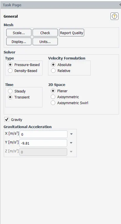
No turbulence model is checked as this comes under the laminar regime.
As we are dealing with two phases, multi-phase modeling i.e, the Volume of fluid model with implicit method, has to be applied.
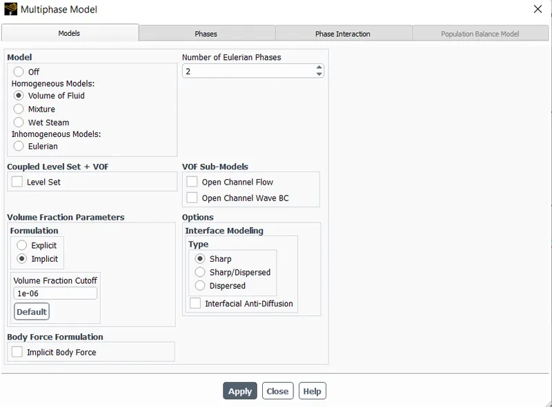
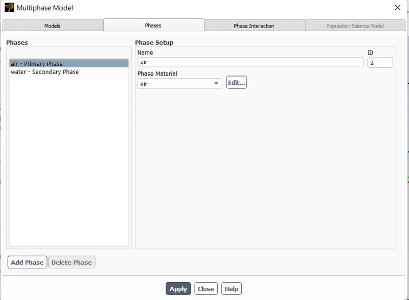
Then, the phases are specified with the primary phase as air and the secondary phase as water. Before this step, the water properties should be extracted from the fluent database in Create edit materials.
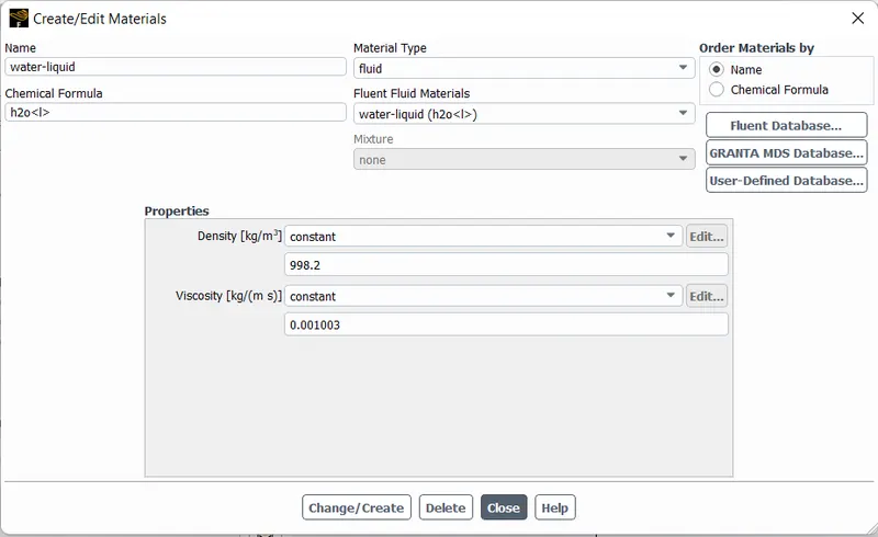
Then for the initialization of the flow variables, the standard initialization method is used.
After initialization patching of the phases is done.
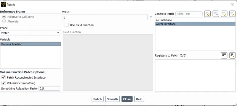
The air phase is given a volume fraction of 0 and the water phase is given a volume fraction of 1.
Then the contour of phases and solution animation are created.
step-4 solving and results :
Now, we initially run the solver for 100 timesteps, size of each time step - 0.005s to check whether the physics is being evolved.
case-1 :
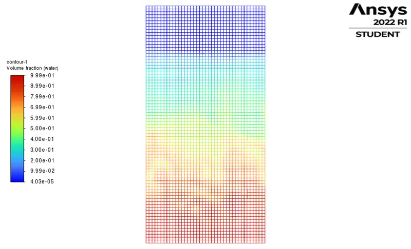
contour of phases
Animation video
case-2:
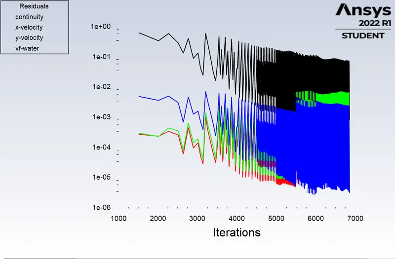
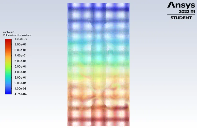
contour of phases
Animation video
case-3 :
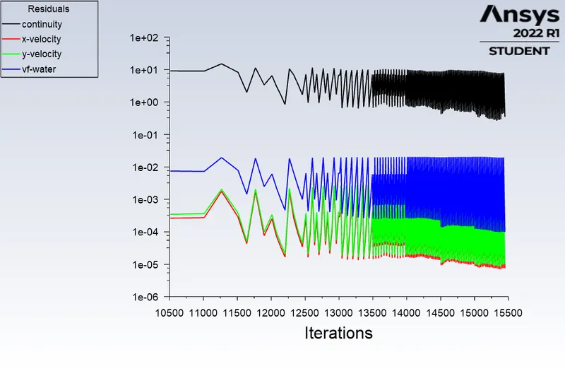
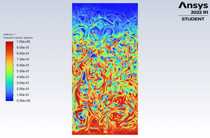
contour of phases
Animation video
NOTE:
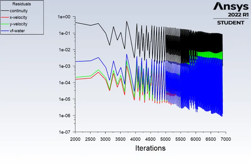
When the solver was run with a time step size of 0.005s, the floating-point error showed up pointing towards the divergence of the solution which might be due to various factors. One of the most important factors is the CFL criterion,
CFL number = alpha*dt/dx^2 <=0.25 (for stable solution)
When the mesh is refined, due to the decrease in the mesh size, the solution blows up/diverges. So, to make up for this change, the size of the time step is decreased from 0.005s to 0.001s. Then the solution does not diverge and the physics evolves.
case-4 :
To capture the instabilities(refined mesh) with user-defined fluid with properties density = 400 kg/m^3 and viscosity = 0.001 kg/m-s as the lighter fluid and water as the heavier fluid .
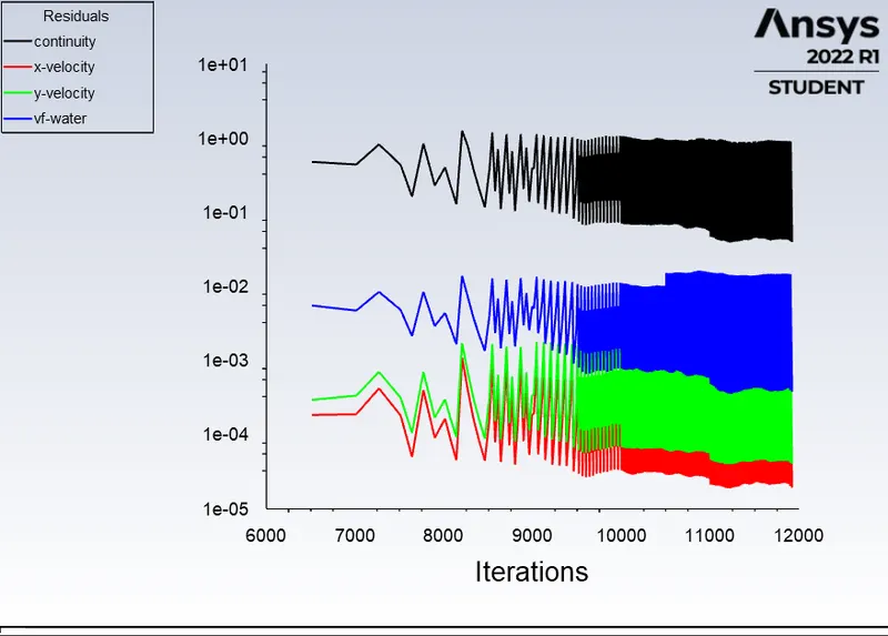
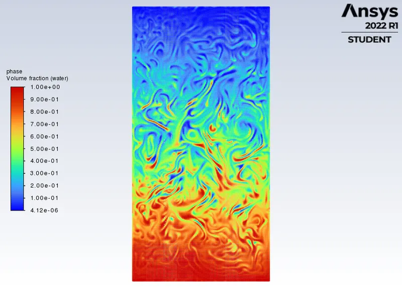
contour of phases
Animation video
The Atwood number (A) is a dimensionless number in fluid dynamics used in the study of hydrodynamic instabilities in density stratified flows. It is a dimensionless density ratio defined as

 = density of the heavier fluid
 = density of the lighter fluid
Atwood number for cases 1,2,3: A=1000-1.22/1000+1.22 = 0.9975
Atwood number for the case 4: A = 1000-400/1000+400 = 0.4285
Conclusion :
1. When the mesh size was decreased, the instabilities were captured accurately.
2. With the decrease in the mesh size and time step in case3, the turbulent mixing was captured clearly and the computation power increased significantly.
3. The time step has to be chosen considering various factors, in which the CFL criterion is the most important factor. If not the solution diverges.
4. When the Atwood number is near 1 (i.e, for cases 1,2, and 3), the interface deforms faster, then the turbulent mixing happens while the denser fluid starts to settle down at the bottom and the less dense fluid moves up and stabilizes at a faster rate.
5. But when the Atwood number is near zero, the deformation of the interface and stabilizing happens at a slower rate.