Week 1- Mixing Tee

Aim:

1. To perform steady-state simulations to observe the flow field inside the T-junction geometries(both long and short). The reason for this experiment is that, inside the T-junction, due to the different temperatures at inlets(hot and cold inlets), can lead to temperature fluctuations at the adjacent walls.

2. To apply the k-epsilon and k-omega SST turbulence models, and choose the better turbulence model for this application.

3. To perform grid independent study for any of the cases.

4. To observe and analyze the effect of length and momentum ratio on the mixing effectiveness in both the geometries.

Introduction:

A T-junction pipe is a temperature controlling device that has two inlets and one outlet. Out of the two inlets, chilled air is passed through one of them while hot air is passed through another, the outlet is where we want the desired temperature as shown below.

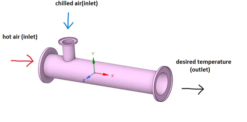
The thermal mixing phenomenon, which occurs due to different temperature inlets, leads to transient temperature fluctuations at the adjacent pipe walls, cyclic thermal stresses in the pipe walls, and consequently to thermal fatigue and failure of the
pipeline. Thus monitoring the temperature field inside the T-junction geometry has immense importance.

In any CFD analysis, the workflow that is followed is

Setting up the geometry ----> Meshing ----> setting up the solver ---->solving ---->post-processing results

step-1 Setting up the geometry :

First, we import the pre-designed T-junction geometry to Spaceclaim where editing is done based on our requirements. The pre-designed geometry has a thickness around the flow region. In this CFD analysis, we want to observe the flow field inside the T-junction geometry. So, we extract the volume inside the T-junction pipe by a feature called Volume Extraction.

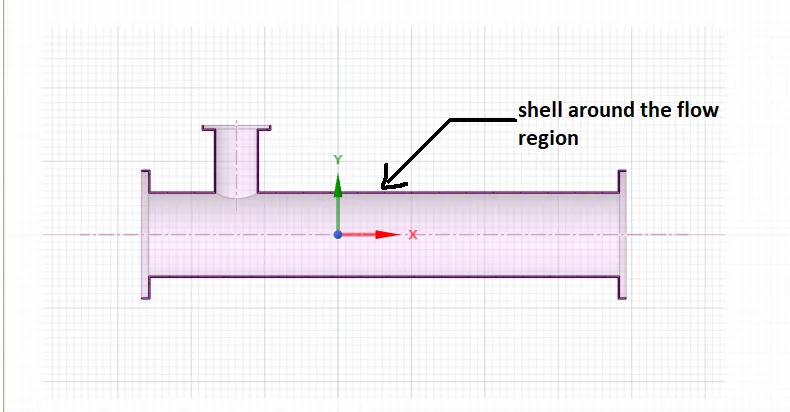
sectional view of the geometry

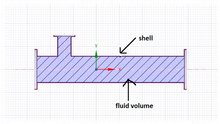
sectional view after extracting the fluid volume

As we are not interested to find the stresses on the walls of the pipe, we suppress the shell by suppressing the shell for the physics option. We will only be working on the fluid volume.

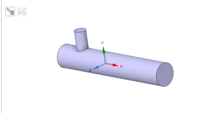
3D view of the fluid volume after hiding and suppressing the shell

step-2 Meshing :

Meshing is basically the process of generating a grid i.e, dividing complex geometries into elements that can be used to discretize a domain. First, a baseline mesh is generated(i.e, without changing any parameters) to check the solver settings. If the flow physics works fine, then the mesh refinement is done. Ansys uses a Bounding box approach i.e, it assumes the smallest box to which the geometry can be fitted, to create this mesh as shown below.

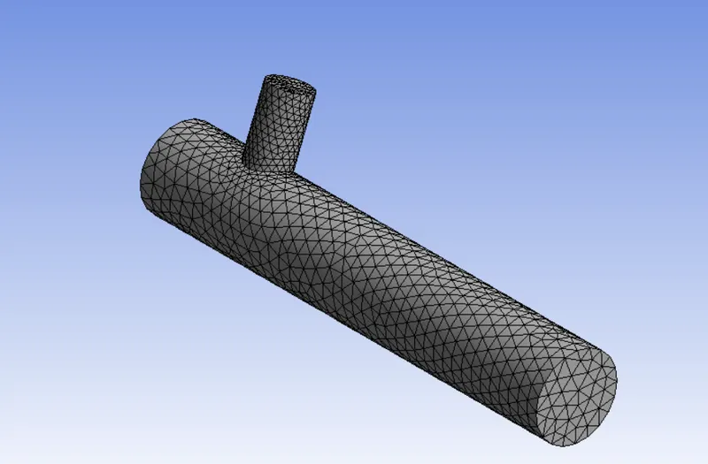
baseline mesh (mesh size =10.219 mm)

nodes =2840

elements=12780

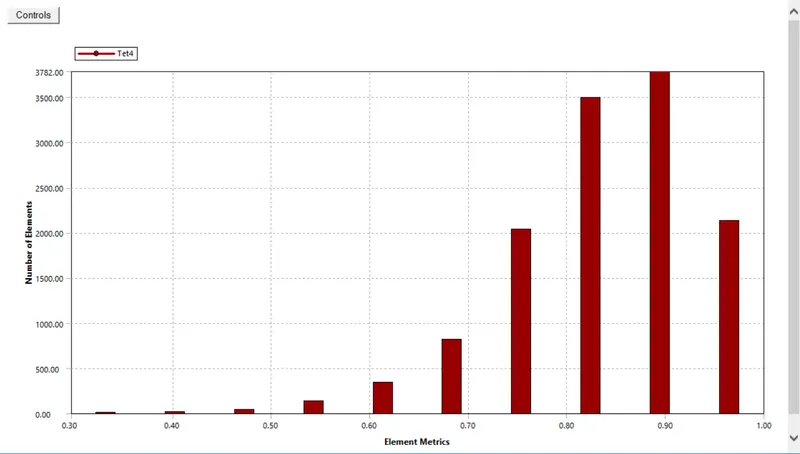
mesh quality

To check the quality of the baseline mesh, the mesh metrics option is changed to element quality in mesh settings.

Most of the elements fall under 0.90(1 being the perfect Tet4-shaped element)and the least number of elements fall below 0.40, which is perfectly fine.

Then the boundaries are defined by selecting different faces and naming them accordingly.

Now, we can proceed further to set up the flow physics.

step-3 Setting up the solver in Ansys FLuent:

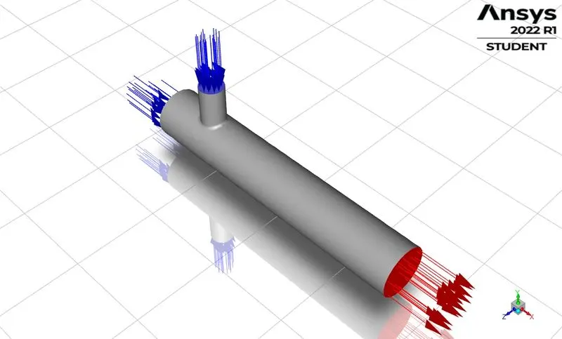
In this step, we define various parameters like initial and boundary conditions, materials used, time steps(for transient), turbulence model, etc which captures the physics to be simulated.

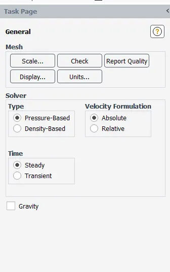
First, we set up the physics by choosing the pressure-based solver which was particularly designed for low-speed incompressible flows(low Mach number), while the density-based solver was mainly designed for high-speed compressible flows(high Mach number).

Then, the steady-state solver is checked, as we are interested in seeing the final results after the flow variables become steady. Along with the standard governing PDE's, we will also be solving the Energy equation.

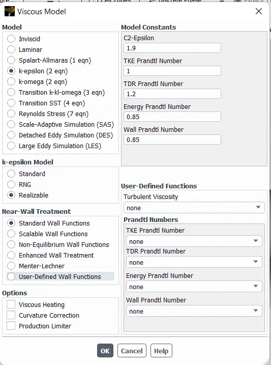
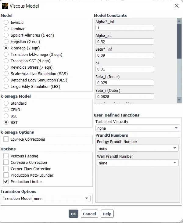
The next parameter that we need to set up is the turbulence model. Initially, we start with both the K-epsilon and K-omega SST models. Based on the results we choose an appropriate turbulence model for the other cases.

The boundary conditions are defined as

cold-inlet : velocity magnitude-6m/s Temperature:19 c

hot-inlet : velocity magnitude-3m/s Temperature:36 c

outlet : pressure outlet

Hybrid initialization is chosen for initializing the domain. Hybrid Initialization is a collection of recipes and boundary interpolation methods. It solves the Laplace equation to produce a velocity field that conforms to complex domain geometries, and a pressure field that smoothly connects high and low-pressure values in the computational domain. So, Hybrid initialization basically works on potential field theory.

Turbulence Modelling:

k-epsilon and k-omega SST turbulence models both work on RANS, in which the flow variables are decomposed into the mean (ensemble-averaged or time-averaged) and fluctuating components and substituted in continuity, momentum, and energy equations which have to be solved. But after averaging the governing equations additional Reynolds stress term appears that represents the effects of turbulence.

To model this stress term, Boussinesq hypothesis is used. The Boussinesq hypothesis is used in the Spalart-Allmaras model, the k-epsilon models, and the k-omega models. The advantage of this approach is the relatively low computational cost associated with the computation of the turbulent viscosity. In the case of the k-epsilon and k-omega models, two additional transport equations (for the turbulence kinetic energy, k, and either the turbulence dissipation rate, epsilon, or the specific dissipation rate, omega) are solved, and turbulent viscosity is computed as a function of k and epsilon or k and omega.

Step-4 Results :

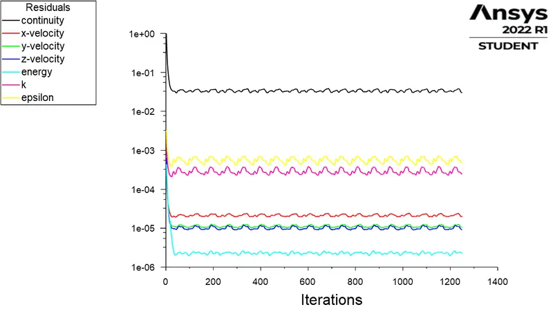
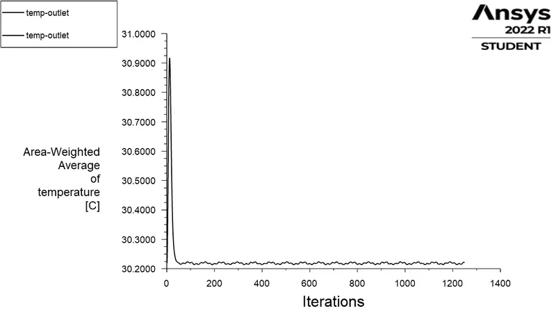
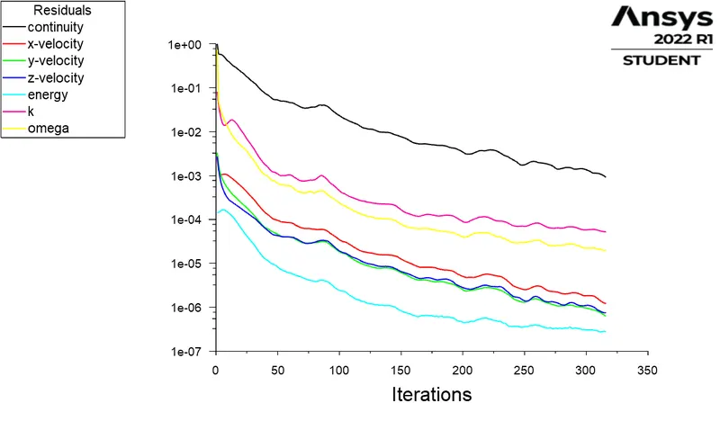
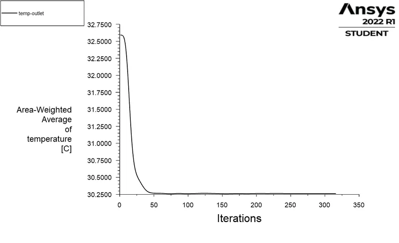
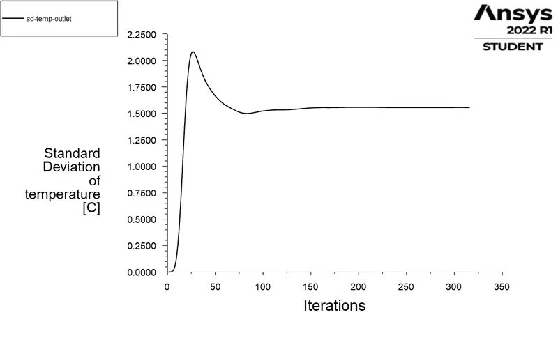
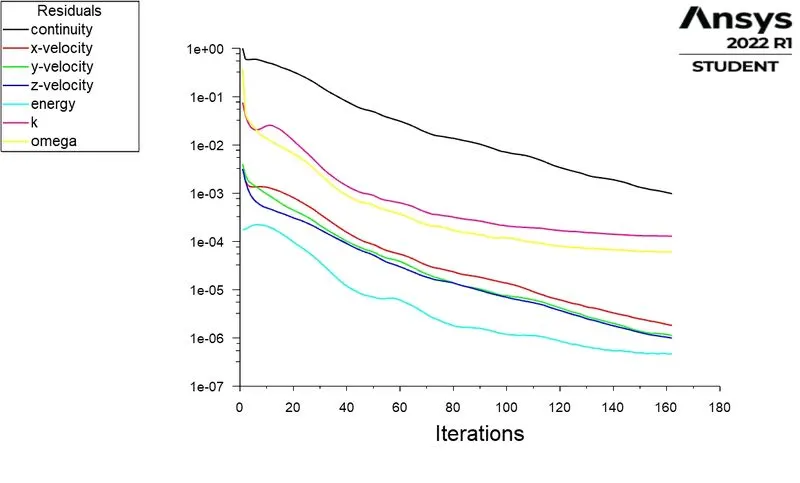
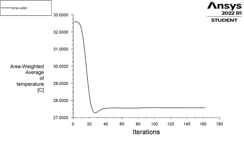
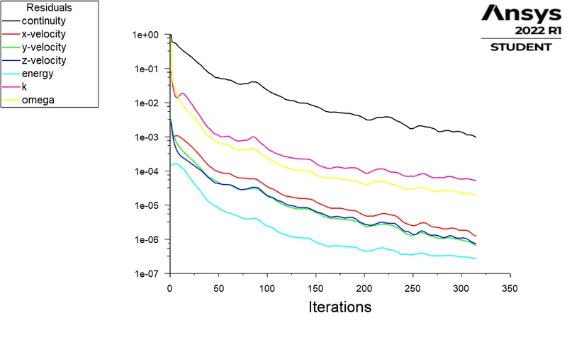
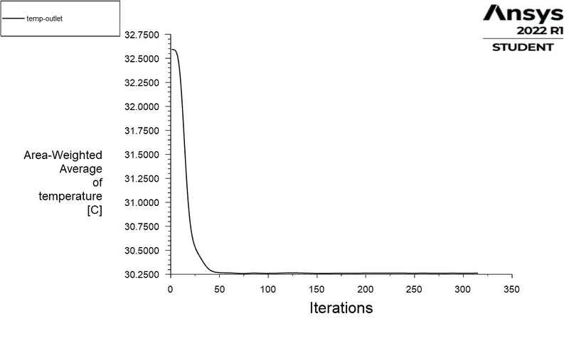
After initialization, the solver is run for a number of iterations, we usually start with around 400-500 iterations and look at the reports and residuals. The convergence is assessed on various aspects like the stability of residuals, reports (in our case the temperature at the outlet, and so on )

long tee (MR=2)		Average outlet temperatures	Standard Deviation of outlet temperature	Convergence(no of iterations)
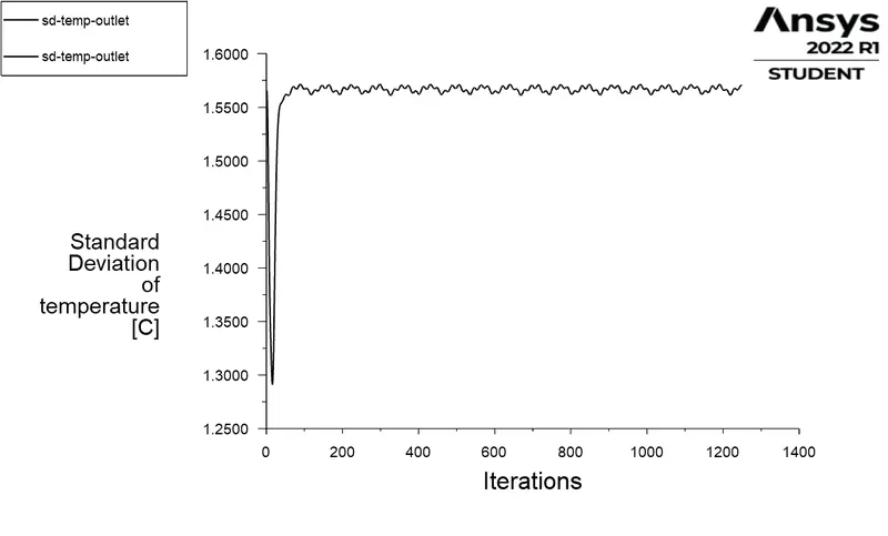
case1	k-epsilon	30.2211	1.570	no convergence after 1250 iterations
case2	k-omega SST	30.2625	1.554	315

Both of the turbulence models point us towards the same outlet temperature, but the number of iterations for the solution to converge varies. Therefore, we proceed to use the k-omega SST turbulence model for our further cases. As the near-wall damping functions in the k-epsilon model are unreliable in a variety of flows.

case1 :long tee(mr=2) k-epsilon

case2 : long tee(mr=2) k omega SST

step-5 Post-processing results :

case-1 :long tee(mr=2) k-epsilon

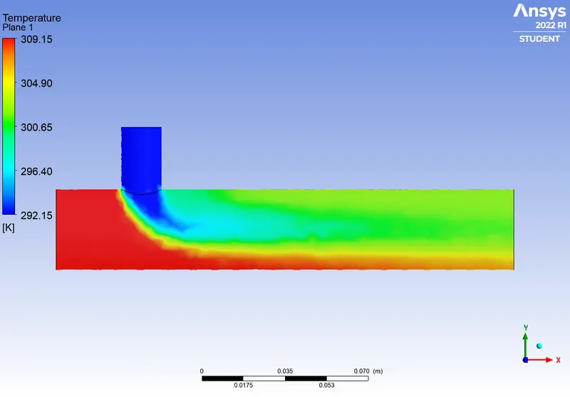
temperature contour across the length of the geometry

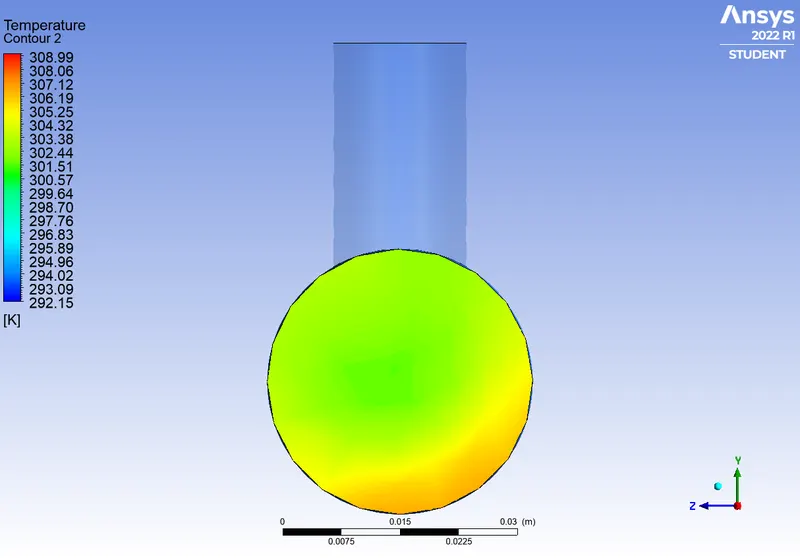
temperature contour at the outlet

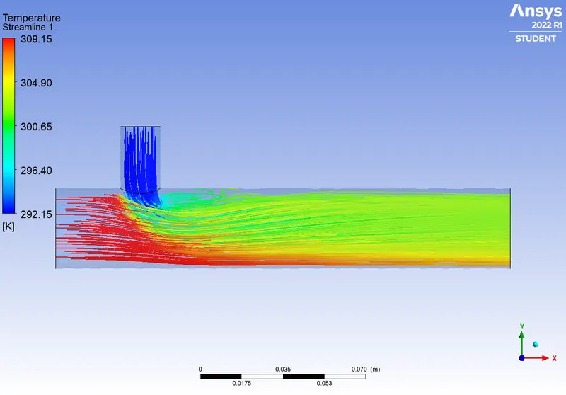
temperature streamlines inside the flow region

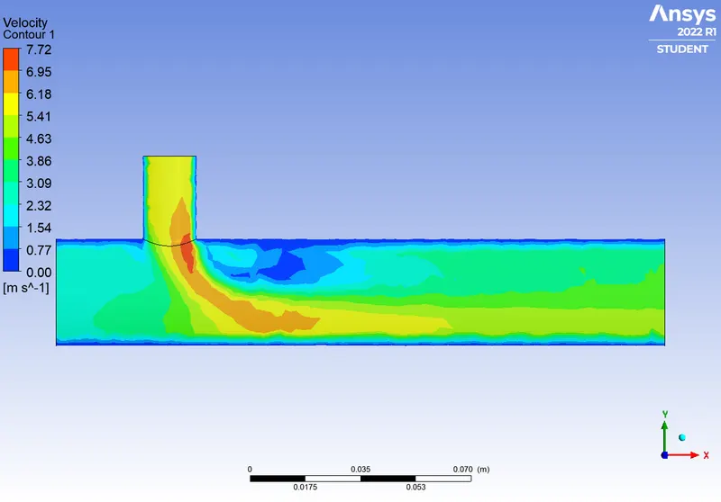
velocity contour across the length of the geometry

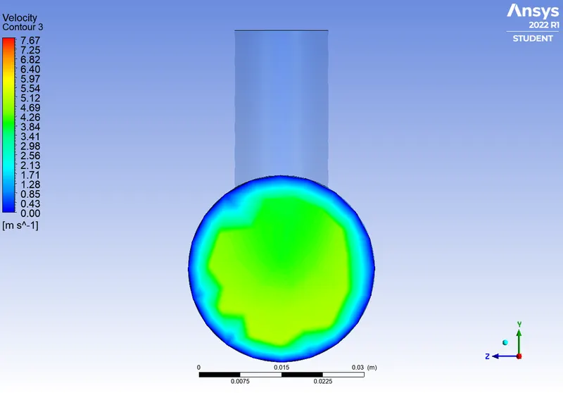
velocity contour at the outlet

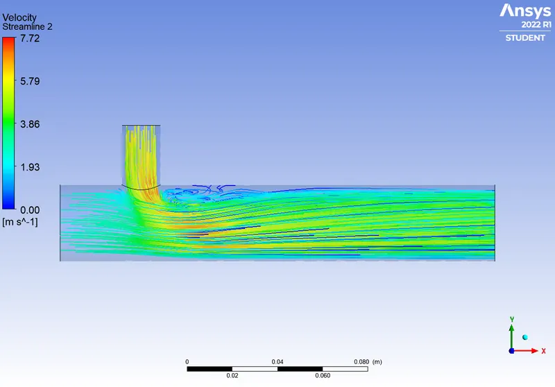
velocity streamlines inside the flow region

case2 : long tee(mr=2) k omega SST

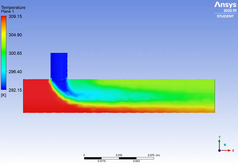
temperature contour across the length of the geometry

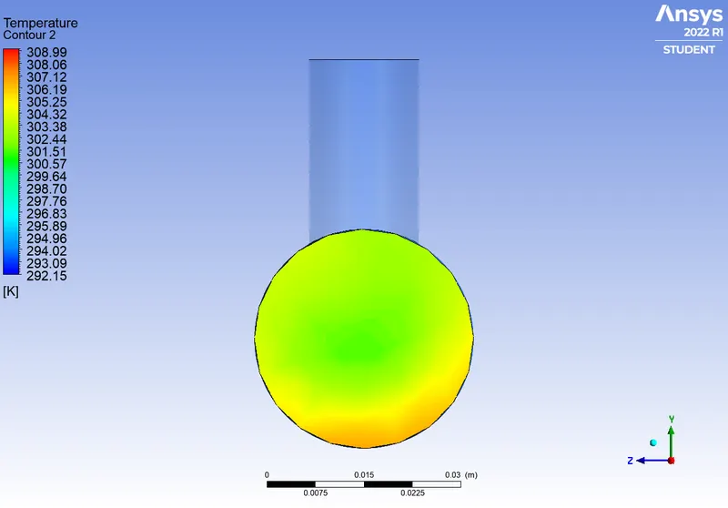
temperature contour at the outlet

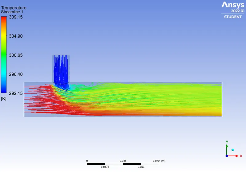
temperature streamlines inside the flow region

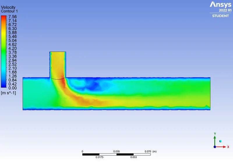
velocity contour across the length of the geometry

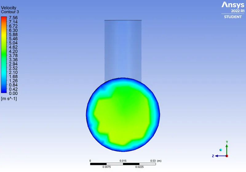
velocity contour at the outlet

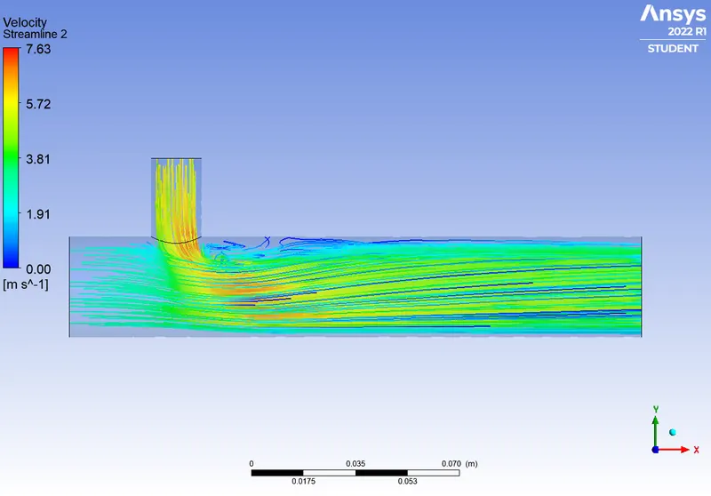
velocity streamlines inside the flow region

Other cases:

case-3: long tee(mr=4)

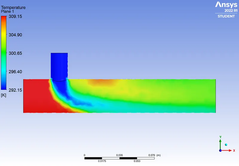
temperature contour across the length of the geometry

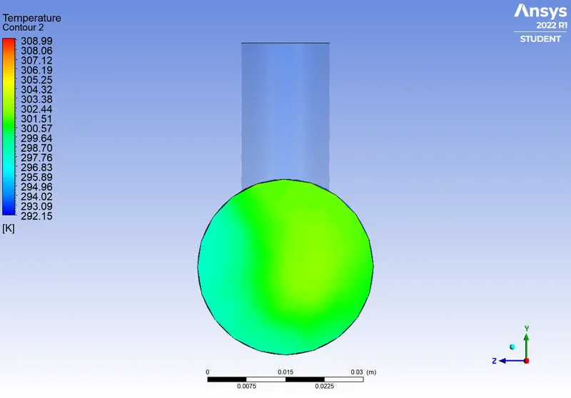
temperature contour at the outlet

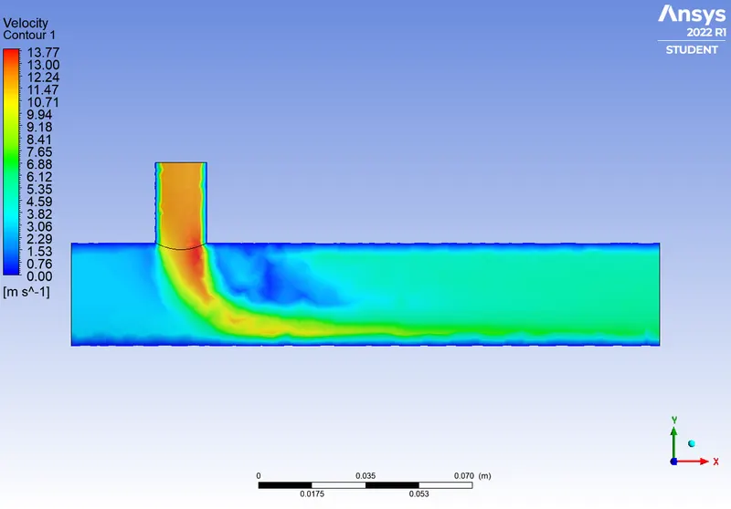
velocity contour across the length of the geometry

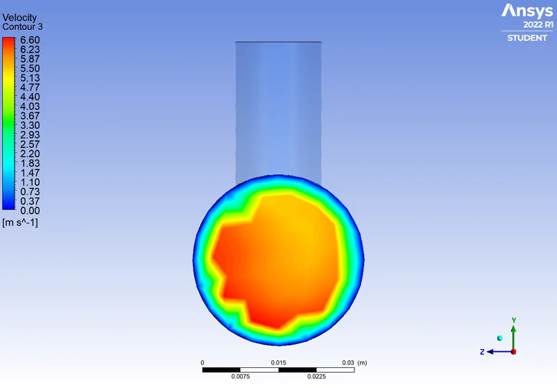
velocity contour at the outlet

case-4: short tee(mr=2)

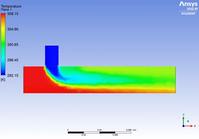
temperature contour across the length of the geometry

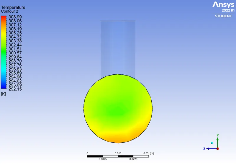
temperature contour at the outlet

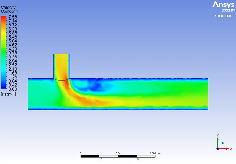
velocity contour across the length of the geometry

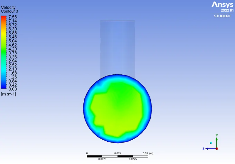
velocity contour at the outlet

case-5: short tee(mr=4)

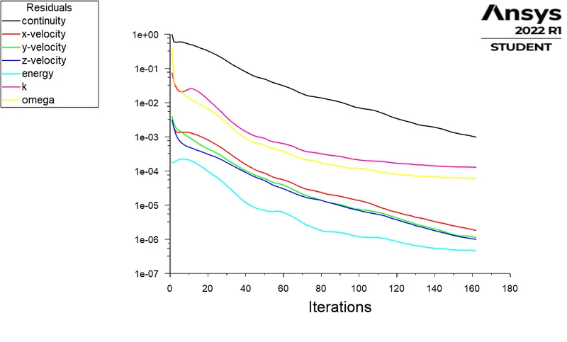
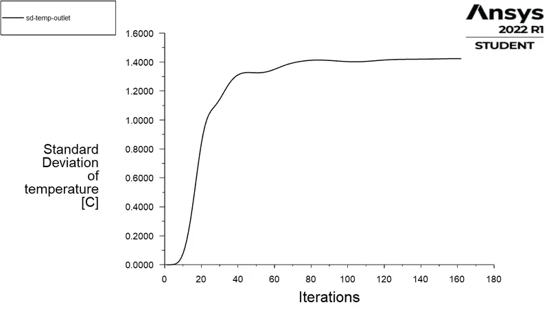
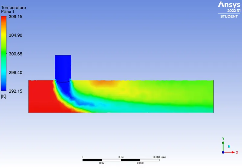
temperature contour across the length of the geometry

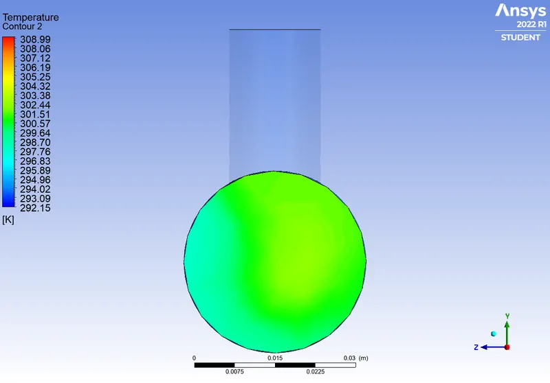
temperature contour at the outlet

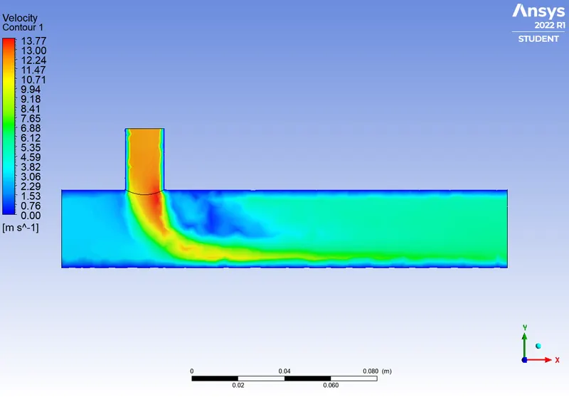
velocity contour across the length of the geometry

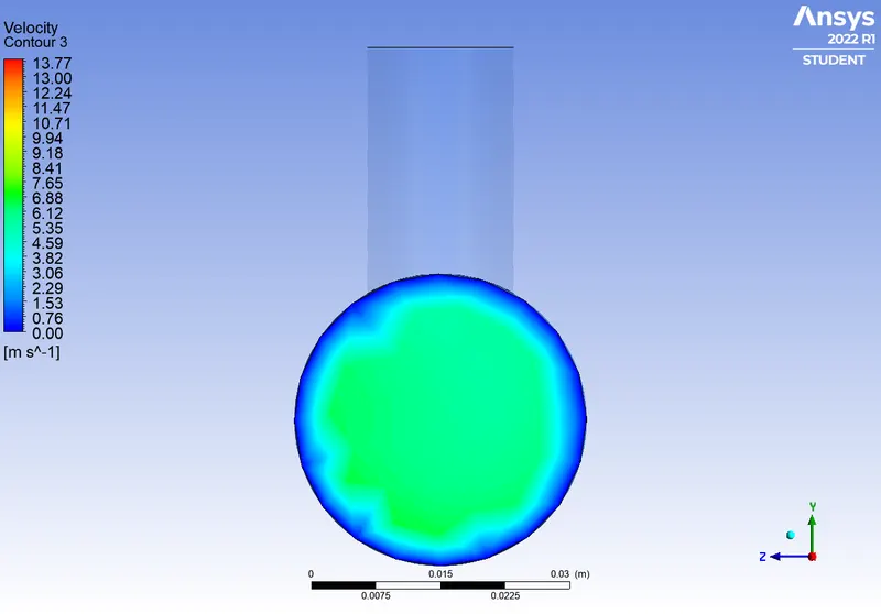
velocity contour at the outlet

Mesh independent study:

Although we are happy that this has "converged" based on Residuals, and Temperature plots. we need to make sure that the solution is also independent of the mesh resolution. Not checking this is a common cause of erroneous results in CFD.

Reducing the element size by half(5mm) and creating inflation layers around the wall:

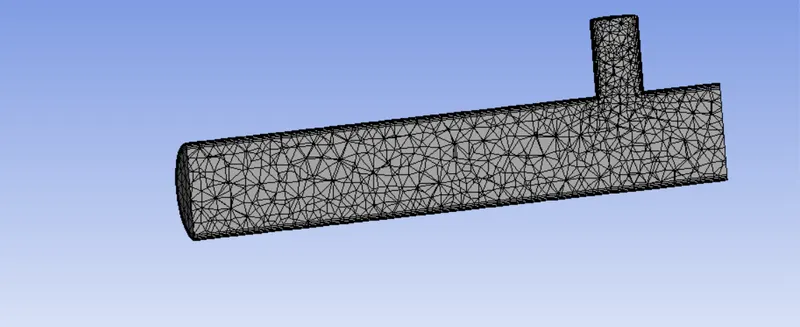
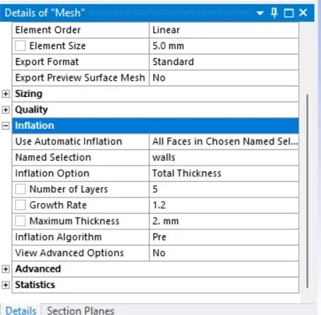
Reducing the element size by half(2.5mm):

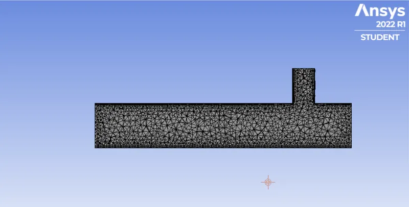
Reducing the element size by half(1.25mm):

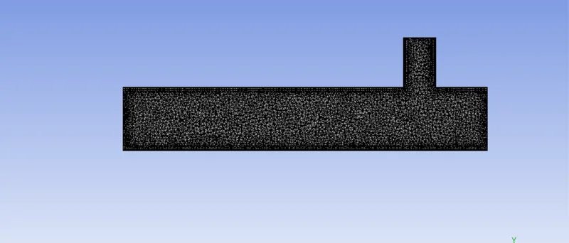
long tee(mr=2)	cells	avg temp outlet	Analytical temperature	sd temp outlet	convergence	nodes
5mm	24090	30.461586	30.80	1.675654	241	9244
2.5mm	86360	30.487526	30.80	2.169962	139	25993
1.25mm	372338	30.46662	30.80	2.309835	162	108628

Even with the change in mesh sizing the outlet temperature is almost the same. But the mesh with an element size of 2.5mm resembles the analytical temperature at the outlet.

Observation:

Analytical solution:

Momentum ratio = 2

mass of hot air =rho*area*velocity=1.225*0.0009*3=0.0033

mass of cold air =rho*area*velocity=1.225*0.0002*6=0.0014

Tmixture=(mass of hot air*temp of hot air + mass of cold air*temp of cold air)/(mass of hot air+mass of cold air)

T1=30.80

Momentum ratio=4

mass of hot air =rho*area*velocity=1.225*0.0009*3=0.0033

mass of cold air =rho*area*velocity=1.225*0.0002*12=0.0029

Tmixture=(mass of hot air*temp of hot air + mass of cold air*temp of cold air)/(mass of hot air+mass of cold air)

T2=28.03

long tee (MR=2)		Average outlet temperatures	Analytical temperature	Standard Deviation of outlet temperature	Convergence(no of iterations)
case1	k-epsilon	30.2211	30.80	1.570	no convergence after 1250 iterations
case2	k-omega SST	30.2625	30.80	1.554	315

	average temp outlet	Analytical temperature	sd temp outlet	convergence(no of iterations)
case-3 long tee(mr=4)	27.5748	28.03	1.423	162
case-4 short tee(mr=2)	30.2625	30.80	1.554	315
case-5 short tee(mr=4)	27.5748	28.03	1.423	162

Conclusion:

1. Even though both of the turbulence models pointed towards the same outlet temperature, the k-omega SST model is preferred to capture the physics near-wall.

2. With the momentum ratio of 2, both the short and long T-junction geometries showed the same outlet temperature. So, short T geometry shows better mixing effectiveness.

3. With the momentum ratio of 4, both the short and long T-junction geometries showed the same outlet temperatures.So, short T geometry shows better mixing effectiveness.

4. We can finally conclude that short T is better than long T geometry in comparison to the mixing effectiveness.