Week 4.1 - Linear convection for varying the number of nodes

Aim :

To solve the one-dimensional linear convection equation which partly resembles the governing momentum equation in Matlab. And to analyze how the solution changes with changing the number of nodes.

MATLAB code :

%solving linear convection equation
%du/dt + c*du/dx=0
close all
clear vars
clc

%inputs
L=1;               % length of the domaain
c=1;               %  Constant convection coefficient
dt=0.01;           % time step
%n=160;
nn=[20,40,80,160]; % number of nodes/grid points


for w=1:length(nn)
    n=nn(w);
    x=linspace(0,L,n); % creating the domain
    dx=x(2)-x(1);      % element size
    nt=40;             % number of time steps

    %initialize arrays
    u=ones(1,n);
    n_start=0.1/dx + 1;
    n_end=0.3/dx + 1;
    u(n_start:n_end)=2;
    u_initial= u ;

    %Applying boundary conitions
    u(1)=1;
    uold=u;       % assigning uold as the initial array


    %solving the equation ( time loop)
    for j=1:nt
        for i=2:n % space loop


            u(i) = -c*dt/dx*(uold(i)-uold(i-1))+uold(i);

        end

        uold = u; % updating the old values

        figure(w)
        subplot(2,1,1);
        plot(x,u_initial);
        xlabel('x');
        ylabel('velocity');
        axis([0 1 0 2]);
        subplot(2,1,2);
        plot(x,u);
        axis([0 1 0 2]);
        xlabel('x ');
        ylabel('velocity');
        pause(0.01);

     
    end
end

one dimensional linear convection equation:

∂u/∂t + c (∂u/∂x)=0

discretization of the above equation

Using first-order forward differencing for the time derivative and first-order backward differencing for the space derivative in the equation.

u(i)-uold(i)/dt + c*[uold(i+1)-uold(i)]/dx = 0 -------> explicit method ( As we are computing with the information from previous time step)

u(i)-uold(i)/dt + c*[u(i+1) - u(i)]/dx = 0 -----------> implicit method ( As we are considering the information from current time step)

The above-discretized equation is integrated over time known as the time-marching method.

Defining and Initialising the domain

length of the domain = 1m

Dividing the domain into nodes. So that the above equation can be solved at each node and move forward across the domain.

The domain is divided into nodes by ' linspace ' cmd

syntax : linspace(x1,x2,n) generates n points between x1 and x2

Initial condition/array :

We want to assign velocity values at every node of the domain or We want to create an initial velocity profile.

constant convective coefficient =1

Applying Boundary conditions :

The boundary value for each and every velocity profile is set to 1 m/s.

Solving the explicit equation:

u(i)-uold(i)/dt + c*[uold(i+1)-uold(i)]/dx = 0

the initial array u is assigned as uold

for loop is used to calculate the u at each value of i and i = 2:n ---> the value of u is calcuated across the domain(space loop)

Then u array is calculated at each time step using for loop j=1:nt nt-number of time steps ( time loop)

when moving from one time step to another, the u array which we calculated at the current time step becomes the old u array for the next time step.

so, we assign uold as u.

As we want to analyze how the results vary with the number of nodes, for loop is used to calculate the result (u array at every time step) for a particular number of nodes 'n'. w is the loop variable for changing the nodes w=1:length(nn)

nn=[20,40,80,160] -----> different values of nodes

plotting:

The objective is to compare the initial and final profiles (for a different number of nodes).

so plot(x,u_initial) is used as the initial plot.

As u array changes with time, we need to plot u after each time step.

So, plot(x,u) is placed inside the time loop.

xlabel('x') ---------> used to label the x-axis as x .

ylabel('velocity')-----> used to label the y-axis as velocity.

'axis([a b c d])' --------> used to fix the axis . the x-axis is fixed from a to b and the y-axis is fixed from c to d.

pause(0.01) -----------> used to pause the plot for 0.01

subplot(m,n,p) -----------> used to break the figure window into mxn subplots. p is used to define the current subplot.

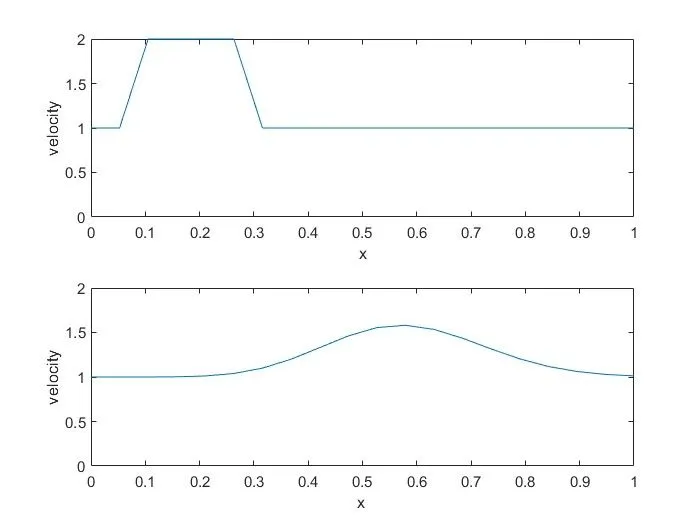
number of nodes=20

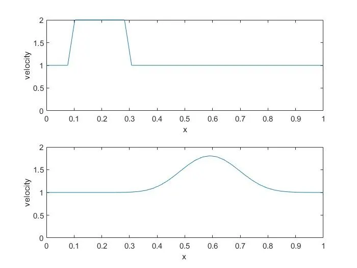
number of nodes= 40

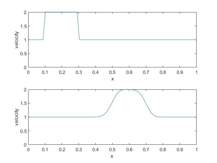
number of nodes=80

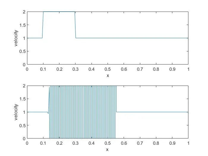
number of nodes = 160

the first figure in each case is the initial velocity profile

the second figure in each case is the velocity profile after 40-time steps, each time step dt=0.01 / final velocity profile.

Conclusion :

Numerical diffusion:

Numerical diffusion refers to the amplitude damping of the numerical solution as compared to the exact solution. This occurs as we are ignoring the terms (truncation error) in forward and backward differencing schemes for time and space derivatives.

1.The RHS is the truncation error for convection equation, v is the CFL number (v) [v= u * dt/dx] ,the coefficient of ∂^2 u /∂x^2 i.e, (a*dx)/2*(1-v) is called the diffusivity coefficient

2. As the number of nodes are increasing, the element size(dx) keeps on decreasing. Accordingly, the CFL number(v) (which is inversely proportional to dx ) keeps increasing.

. As the number of nodes increases, the square wave's diffusion slows down.

4. We can observe that the least diffusivity is in the 3rd case(number of nodes = 80) i.e, the CFL number, in this case, is almost equal to 1.

(when v<1 the diffusivity coefficient is positive and has a diffusive effect.)

5. When there are 160 nodes across the domain, the CFL number is the maximum and exceeds 1. So, the diffusivity coefficient becomes negative and the solution blows up.

(when v>1 the diffusivity coefficient becomes negative and has an amplifying effect and is the cause of instability)

6. Basically increasing the number of nodes slows down the diffusion, but at higher values, the solution blows up.