Week 2 - Flow over a Cylinder.

Aim :

1. To simulate the flow over a cylinder using both steady and unsteady solvers and understand the phenomenon of Karman Vortex Street.

2. To observe and analyze the effect of the Reynolds number on the co-efficient of drag.

3. To understand the convergence criteria.

Introduction:

External flows past objects have been studied extensively because of their many practical applications. For example, airfoils are made into streamlined shapes in order to increase the lifts, and at the same time, reduce the aerodynamic drags exerted on the wings. On the other hand, flow past a blunt body, such as a circular cylinder, usually experiences boundary layer separation and very strong flow oscillations in the wake region behind the body. In a certain Reynolds number range, a periodic flow motion will develop in the wake as a result of boundary layer vortices being shed alternatively from either side of the cylinder. This regular pattern of vortices in the wake is called a Karman vortex street. It creates an oscillating flow at a discrete frequency that is correlated to the Reynolds number of the flow. The periodic nature of the vortex shedding phenomenon can sometimes lead to unwanted structural vibrations, especially when the shedding frequency matches one of the resonant frequencies of the structure. So, analyzing the flow past the cylinder becomes of utmost importance to understand the vortex shedding phenomenon, the effect of the Reynolds number on the coefficient of drag

In any CFD analysis, the workflow that is followed is

Setting up the geometry ----> Meshing ----> setting up the solver ---->solving ---->post-processing results

step-1 Setting up the geometry :

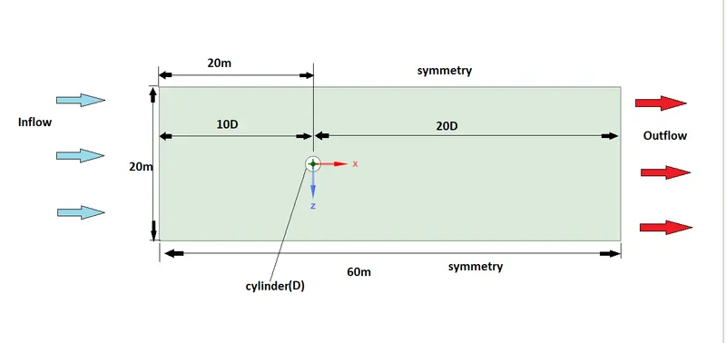
As we are interested in observing the vortex shedding past a cylinder, one plane(XY) of the 3D domain, which consists of a cylinder in the middle(not exactly), is going to satisfy our requirement. To create the geometry, SpaceClaim is used. First, a circle(cylinder) with a diameter(D) of 2m is sketched with the center as the origin. Then the domain is created, using the rectangle cmd, around it with the dimensions, 10D upstream(left side) and 20D downstream(right side) of the cylinder. After the sketching is done, pull cmd is used to create a solid surface from the sketch as shown below.

step-2 Creating the mesh:

Meshing is the process of generating a grid i.e, dividing complex geometries into elements that can be used to discretize a domain. First, a baseline mesh is generated(i.e, without changing any parameters) to check the solver settings. If the flow physics works fine, then the mesh refinement is done.

When the mesh is generated, we automatically get a quadrilateral dominated mesh. But the quad-dominant mesh requires more computation power, as it contains more number of nodes(4 vertices) compared to triangular/tetra mesh(3vertices) in the same area.

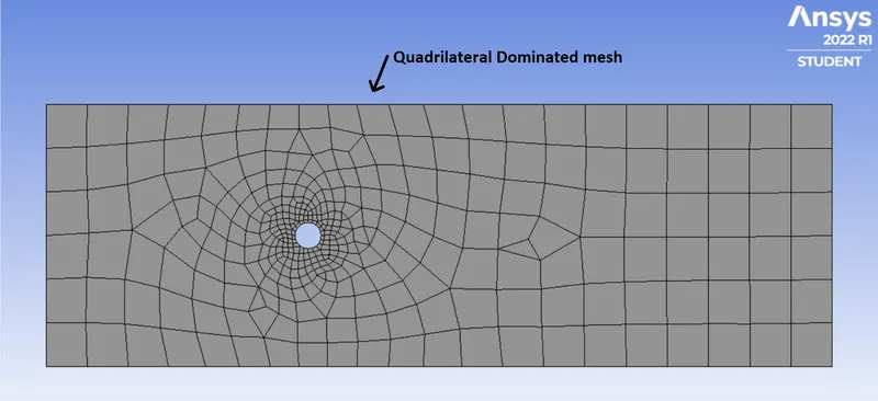
So, we switch to triangular mesh by :

Mesh --> Insert --> Method --> select the geometry --> All triangles method --> generate mesh

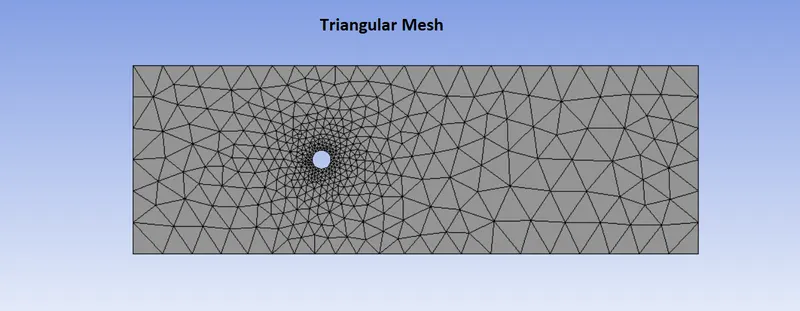
But when we take a closer look at the circle, where the physics has to be captured accurately, it looks like a polygon rather than a circle. In general, when the polygon is made up of infinite edges, it looks like a circle.

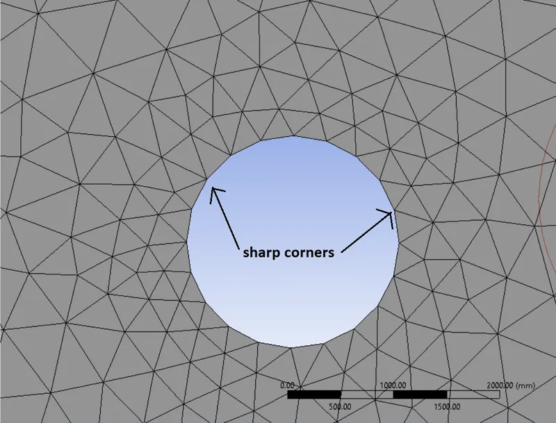
So, we divide the circular edge into a number of divisions by:

Mesh --> Insert --> sizing --> select the circular edge --> type: number of divisions --> number of divisions:36 --> generate mesh

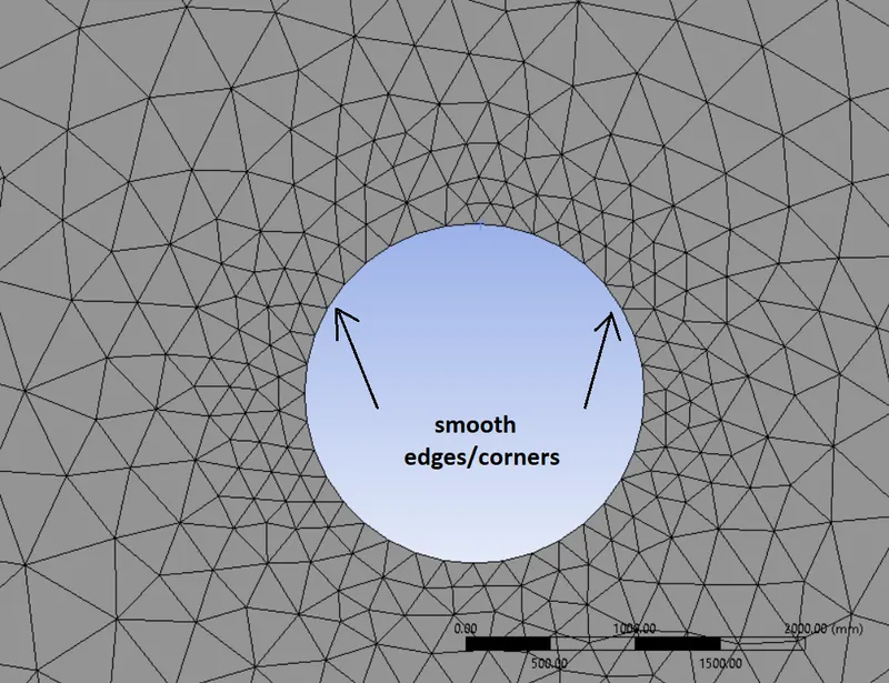
To accurately capture the physics around the body, a body-fitted mesh or creating inflation layers around the cylinder walls will help us do so.

Mesh --> Insert --> Inflation --> select the whole body --> boundary: circle edge --> first layer thickness --> first layer height(5mm) --> Maximum layers(6) --> growth rate:1.2

These parameters indicate that the first layer thickness is 5mm(minimum) and grows adaptively with a rate of 1.2 i.e,

2nd layer height = 1.2*5=6mm

3rd layer height = 1.2*6=7.2mm and so on

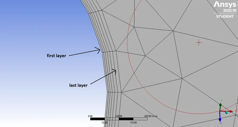
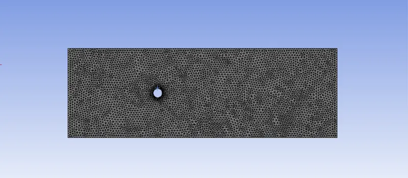
After the mesh refinement, the mesh seems to be coarse with an element size of 3162 mm, 722 nodes, and 1282 elements. So, the mesh is further refined to a mesh with an element size of 500mm,5453 nodes, and 10478 elements.

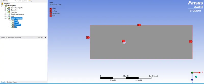
Then the boundaries are assigned by selecting the edges and naming them accordingly as shown below.

Before proceeding any further, we take a look at the quality of the mesh in mesh settings.

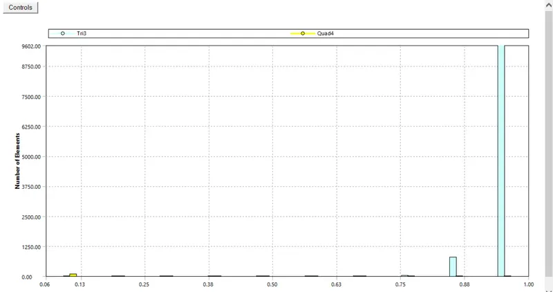
Most of the elements fall above 0.88(1 being the perfect Tri-3 element) which is perfectly fine. Now, we can go ahead to set up the solver in fluent.

step-3 Setting up the solver in Ansys FLuent:

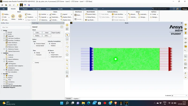
In this step, we define various parameters like initial and boundary conditions, materials used, time steps(for transient), turbulence model, etc which captures the physics to be simulated.

First, we set up the physics by choosing the pressure-based solver which was particularly designed for low-speed incompressible flows(low Mach number), while the density-based solver was mainly designed for high-speed compressible flows(high Mach number).

Both steady and transient state analyses are done. As we are interested in observing the vortex shedding in the laminar regime, the turbulence model is set to laminar.

In this study, we will be working with a user-defined fluid with a density of 1 kg/m3 and viscosity varies with a change in Reynolds number.

Then the boundary conditions are defined, velocity inlet as 1m/s, outlet as pressure outlet, and walls with the no-slip shear condition.

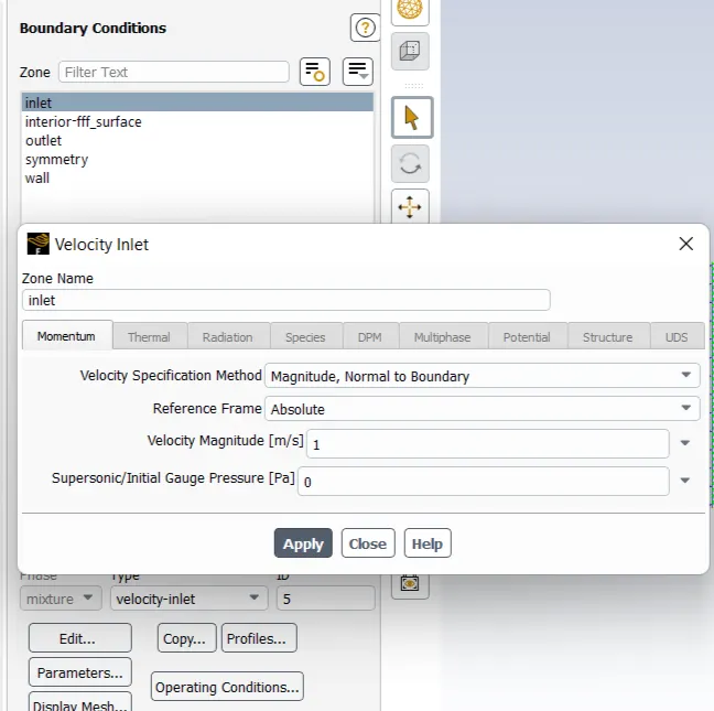
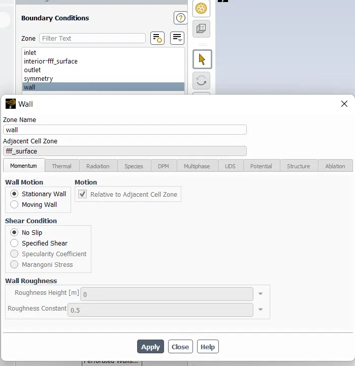
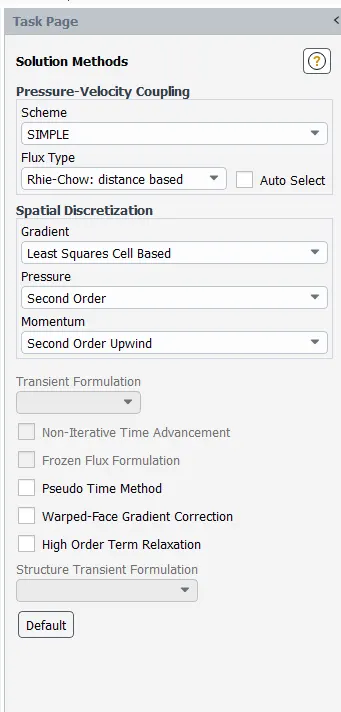
SIMPLE scheme is used in the solution methodology that is going to be implemented.

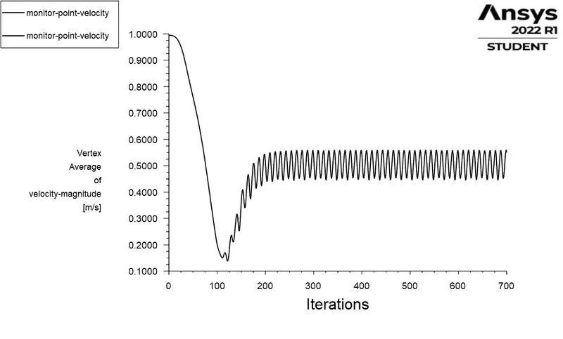
A monitor point at a distance of 10m in the wake region is created. Then using this point, a report definition, to monitor the velocity, is created.

The convergence criteria are turned off, as the physics could develop after the convergence.

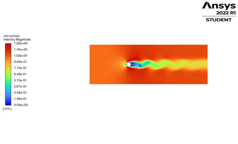
Contour plots of velocity and pressure and Animations are created to visualize the vortex shedding over the iterations/time steps.

Step-4 Solving and Results :

Part-1 Simulate the flow with the steady and unsteady case and calculate the Strouhal Number for Re= 100.

Reynolds number = (density*flow speed*characteristic length)/dynamic viscosity

when Re=100 --> density=1 ; inlet velocity=1 ; characteristic length =D=2 ; dynamic viscosity(mue)=0.02

case-1: steady-state analysis

velocity contour

Observations:

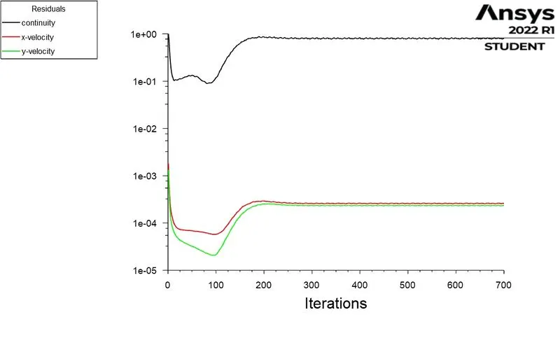
In steady-state analysis, we can observe the vortex shedding phenomenon from the velocity contours as well as from the velocity plot of the monitor point present in the wake region. The residuals fall up to 200 iterations and then it stabilizes and from then no change/oscillations are seen.

The other aspects to be considered to check whether the convergence has been met are the reports which we are interested in i.e, velocity plot at the monitor point.

Even the velocity plot follows a similar pattern after 200 iterations and it does not go up and down i.e, the mean of the oscillations is maintained. So, we can conclude that the solution converges after 200 iterations.

case-2: transient-state analysis

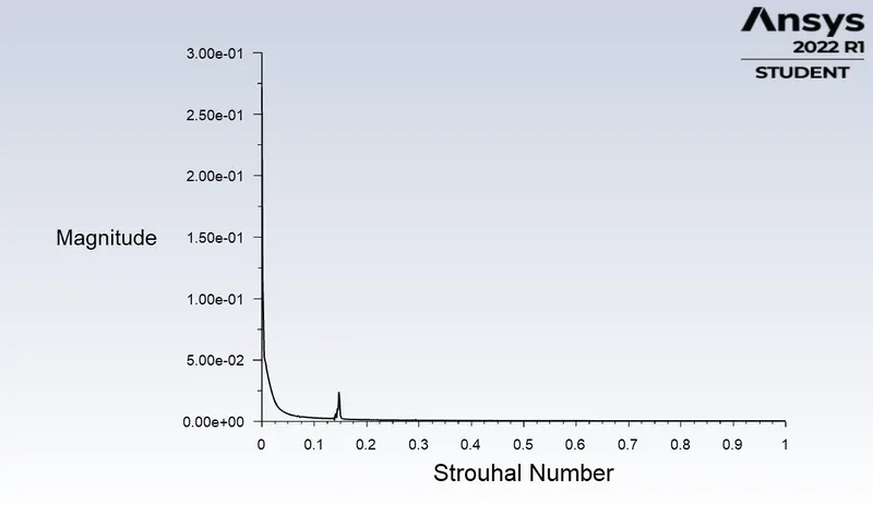
Strouhal number = frequency of vortex shedding*characteristic length / flow velocity

The Strouhal Number forms an important parameter when analyzing unsteady, oscillating flow problems.

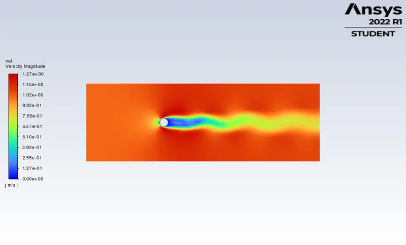
velocity contour

Observations:

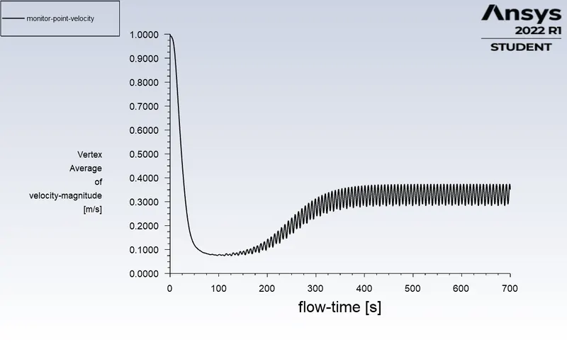
We can observe the vortex shedding phenomenon from the velocity contours as well as the velocity plot of the monitor point present in the wake region.

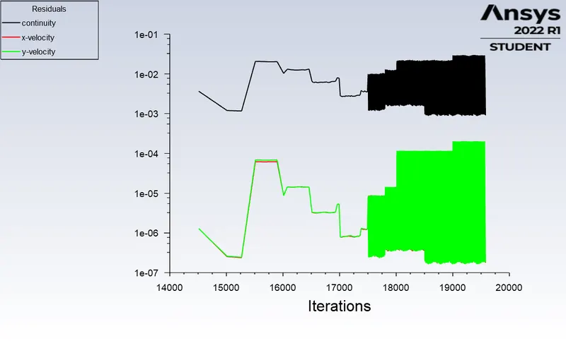
When we observe the residuals plot, the residuals follow a similar pattern after 17500 iterations. The other aspects to be considered to check whether the convergence has been met are the reports which we are interested in i.e, velocity plot at the monitor point.

The velocity plot follows a similar pattern after a run time of 400s and doesn't fall or go up from then. So we can conclude that the solution is converged after 17500 iterations.

Part-2 Calculate the coefficient of drag and lift over a cylinder by setting the Reynolds number to 10,100,1000,10000 & 100000. (Run with a steady solver)

Reynolds number =density *velocity*characteristic length/dynamic viscosity

part-2	Reynolds number	density	dynamic viscosity	velocity computed	characteristic length(D)	coefficient of lift	coefficient of drag	vortex shedding
case-1	10	1.225	0.045	0.18	2	-0.00027188561	3.3500516	no
case-2	100	1.225	0.045	1.83	2	-0.10720576	1.3072656	yes
case-3	1000	1.225	0.045	18.36	2	0.084258068	0.75827752	yes
case-4	10000	1.225	0.045	183.6	2	0.16786613	0.72575438	yes
case-5	100000	1.225	0.045	1836.7	2	0.11273165	0.61346977	yes

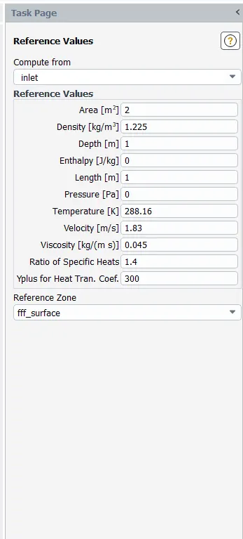
First, the reference values are changed which affects the lift and drag coefficients, particularly the area is changed to 2, and other parameters are computed from the inlet.

Lift force = 1/2* lift coefficient*density*velocity^2*area exposed to the flow

Drag force=1/2* drag coefficient*density*velocity^2*area exposed to the flow

PART-2

case-1 Reynolds number=10

co-efficient of lift

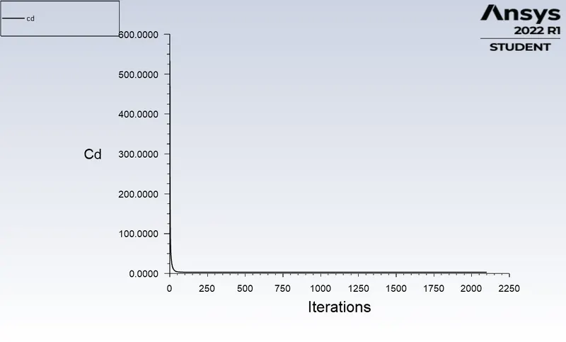
co-efficient of drag

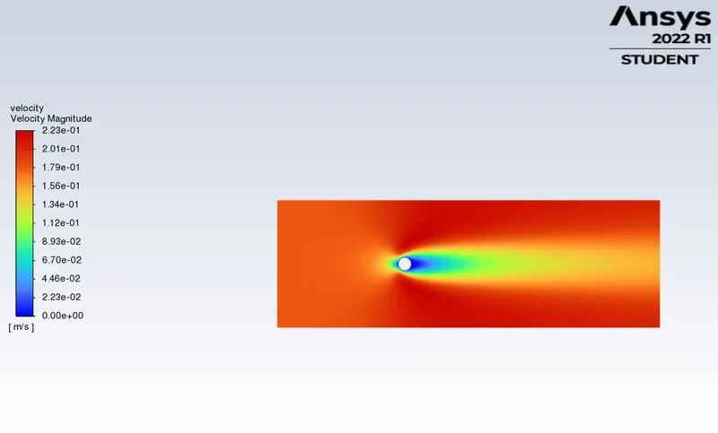
velocity contour

Observations:

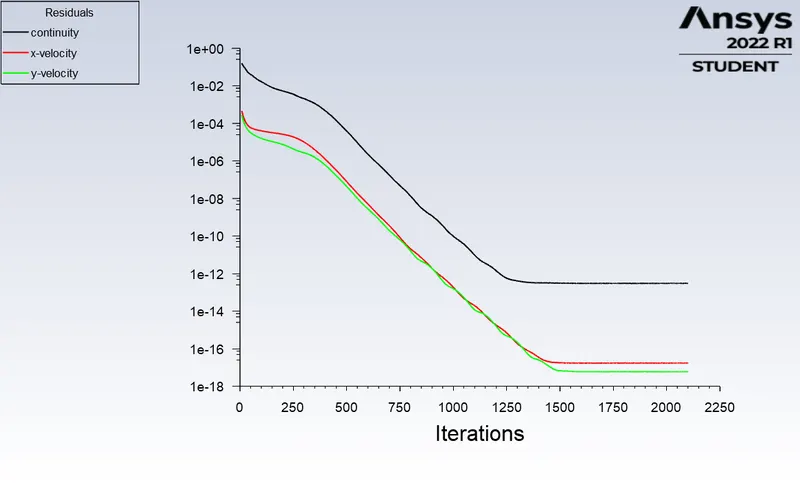
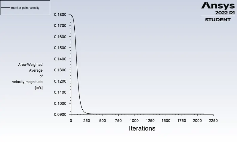
When we observe the residuals plot, the residuals fall drastically up to 1500 iterations approx and then it stabilizes, and we can see no oscillations/change from then. And from the velocity plot of the monitor point present in the wake region, we can infer that there is no vortex shedding happening.

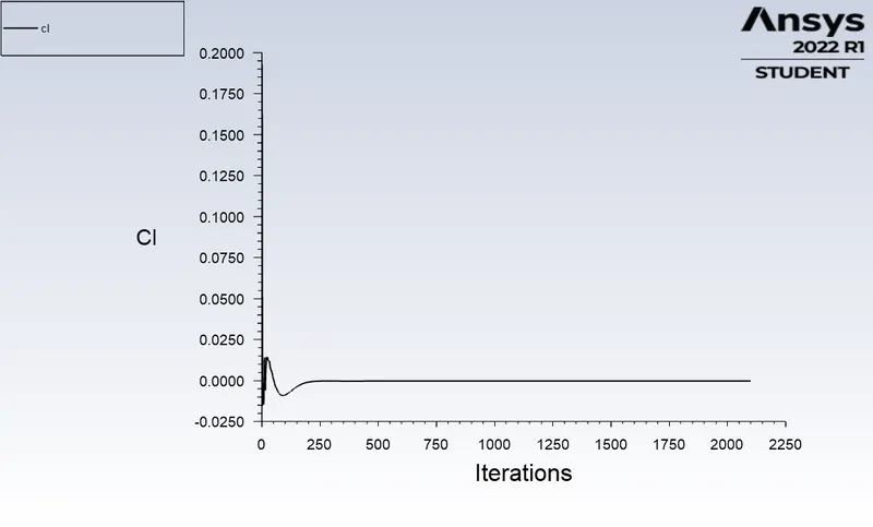
After analyzing the residuals plot, the other aspects that have to be considered for the convergence to meet are the reports that we are interested in i.e, monitor point velocity, lift coefficient, and drag coefficient plots.

The velocity plot becomes quite stable after 250 iterations, and the lift and drag coefficient plots become steady after 150 iterations. So we can conclude that after 1500 iterations the solution has converged.

case-2 Reynolds number=100

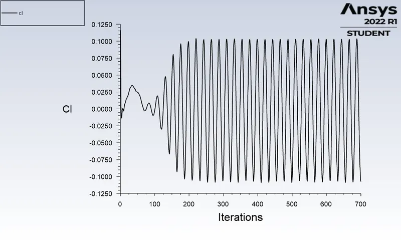
co-efficient of lift

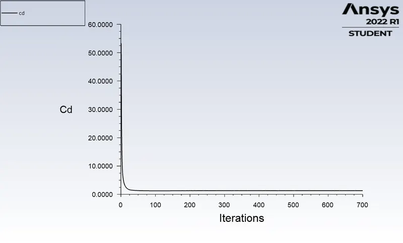
co-efficient of drag

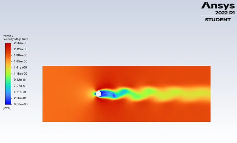
velocity contour

Observations:

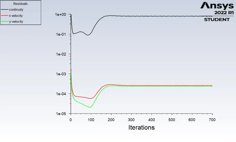
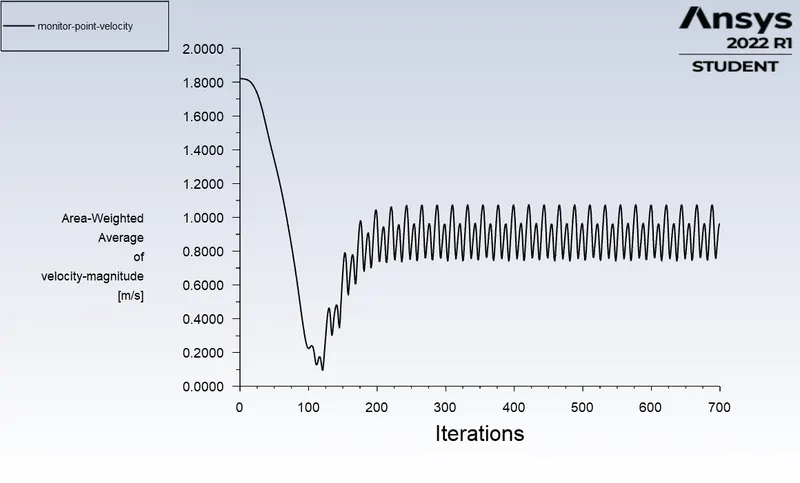
When we observe the residuals plot, the residuals fall up to 100 iterations and then stabilize after 200 iterations approx, and we can see no oscillations/changes from then. And from the velocity plot of the monitor point present in the wake region, we can infer that there is vortex shedding happening.

After analyzing the residuals plot, the other aspects that have to be considered for the convergence to meet are the reports that we are interested in i.e, monitor point velocity, lift and drag coefficient plots.

The monitor point velocity plot follows a similar pattern after 200 iterations as well. The lift coefficient plot oscillates with a similar pattern after 200 iterations whereas the drag coefficient plot is quite stable after 100 iterations. So, we can conclude that the solution has converged after 200 iterations.

case-3 Reynolds number=1000

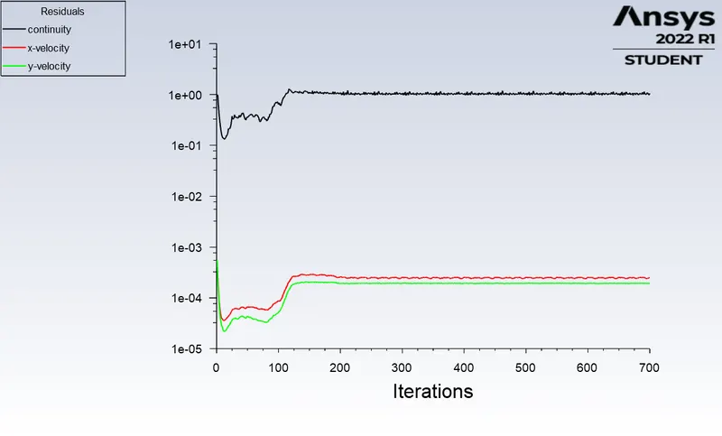
co-efficient of lift

co-efficient of drag

velocity contour

Observations:

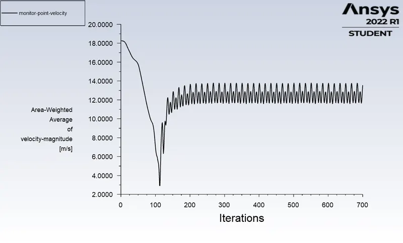
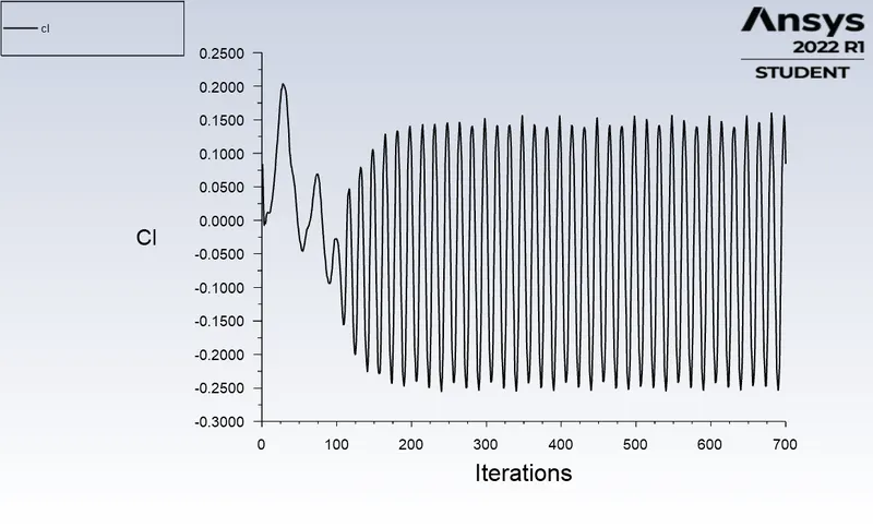
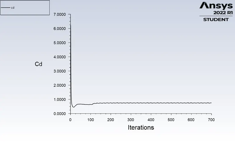
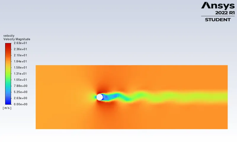
When we observe the residuals plot, the residuals stabilize after 200 iterations approx, and we can see no oscillations/changes from then. And from the velocity plot of the monitor point present in the wake region, we can infer that there is vortex shedding happening.

After analyzing the residuals plot, the other aspects that have to be considered for the convergence to meet are the reports that we are interested in i.e, monitor point velocity, lift and drag coefficient plots.

The monitor point velocity plot follows a similar pattern after 200 iterations as well. The lift coefficient plot oscillates with a similar pattern after 200 iterations whereas the drag coefficient plot is stable with slight oscillations after 100 iterations. So, we can conclude that the solution has converged after 200 iterations.

case-4 Reynolds number=10000

Observations :

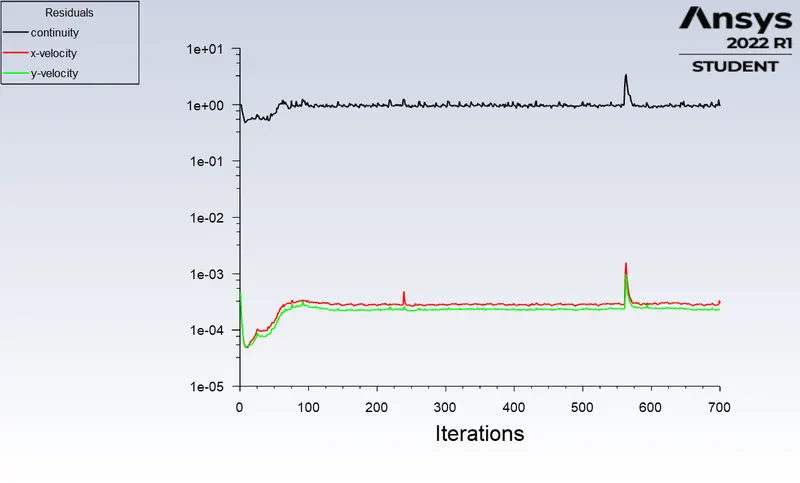
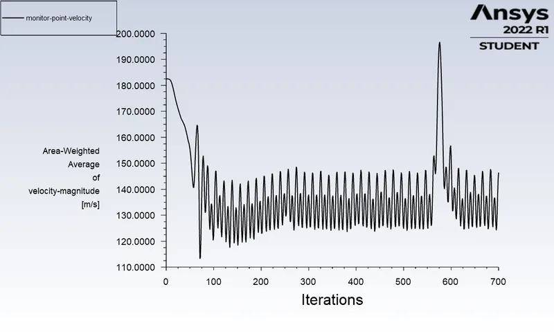
When we observe the residuals plot, the residuals stabilize after 100 iterations approx with slight oscillations. And from the velocity plot of the monitor point present in the wake region, we can infer that there is vortex shedding happening.

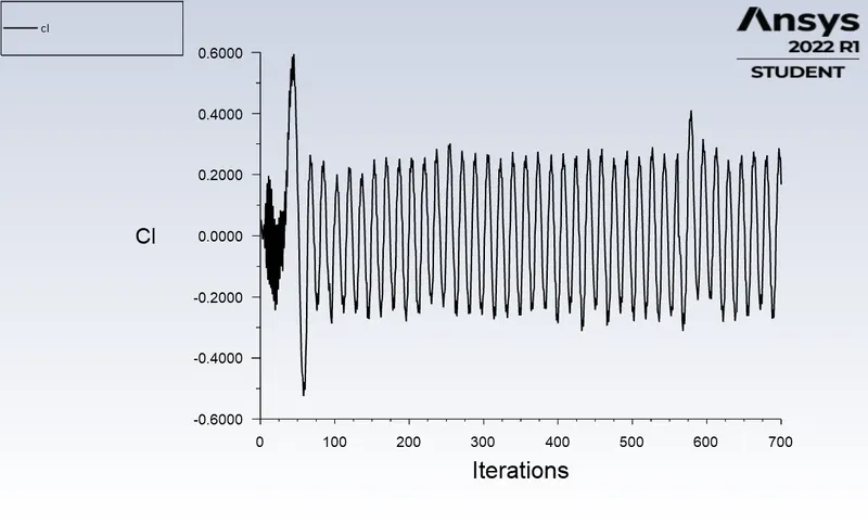
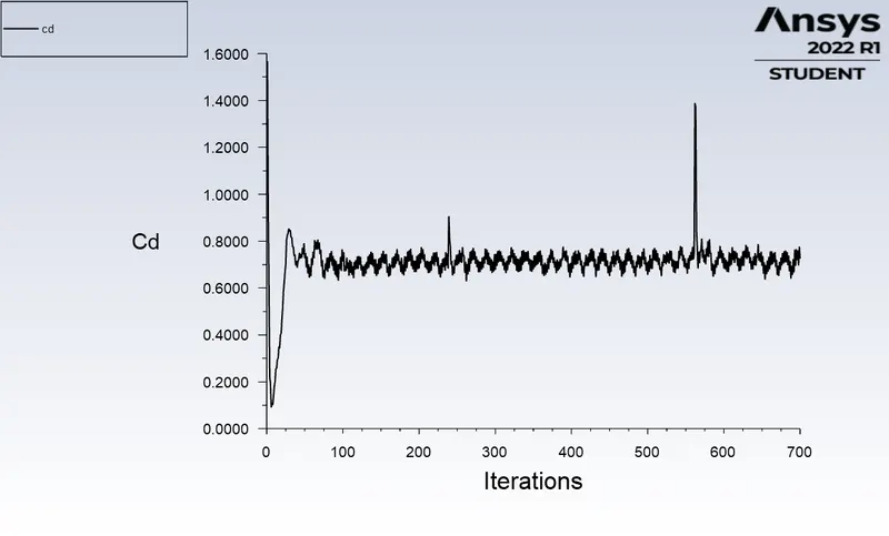
After analyzing the residuals plot, the other aspects that have to be considered for the convergence to meet are the reports that we are interested in i.e, monitor point velocity, lift and drag coefficient plots.

The monitor point velocity plot follows a similar pattern after 100 iterations but the oscillation's mean is not maintained. After 200 iterations, the mean is maintained.

The lift coefficient and drag coefficient plots oscillate with a similar pattern after 100 iterations, with sudden peaks corresponding to the residual plot's peaks. So, we can conclude that the solution has converged after 200 iterations.

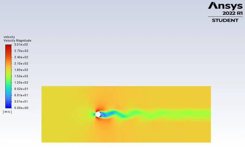
case-5: Reynolds number=100000

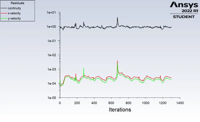
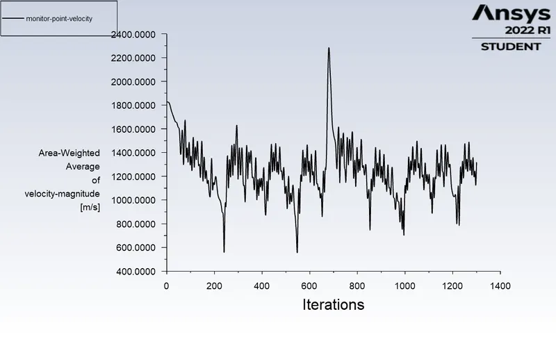
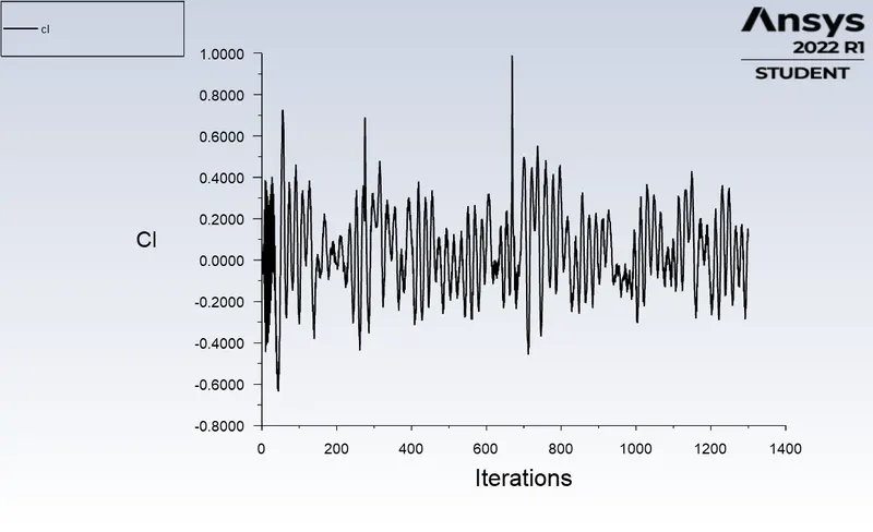
coefficient of lift

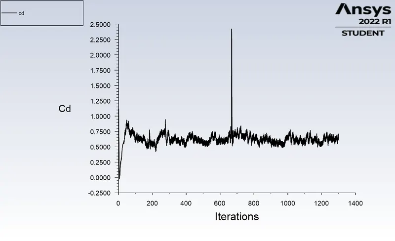
coefficient of drag

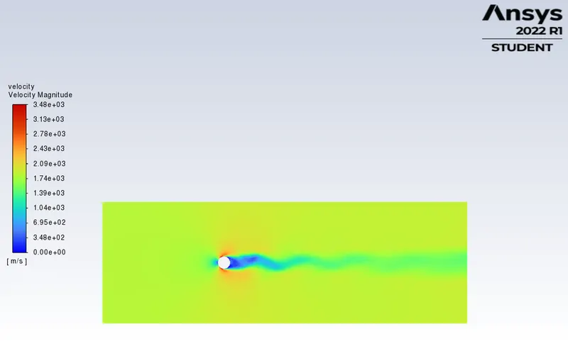
velocity contour

Observations :

When we observe the residuals plot, the residuals oscillate with a similar pattern after 200 iterations approx with sudden peaks in between. And from the velocity plot of the monitor point present in the wake region, we can infer that there is vortex shedding happening.

After analyzing the residuals plot, the other aspects that have to be considered for the convergence to meet are the reports that we are interested in i.e, monitor point velocity, lift and drag coefficient plots.

The monitor point velocity plot follows a similar pattern after 250 iterations approx with sudden peaks corresponding to the peaks in the residual plot.

The lift coefficient and drag coefficient plots oscillate with a similar pattern after 250 iterations with sudden peaks in between corresponding to the peaks in the velocity and residual plots. So, we can conclude that the solution has converged after 250 iterations.

Conclusion:

1. The Von Karman Vortex shedding phenomenon is observed in flow simulations with Reynolds numbers 100,1000,10000,10000.

2. When the Reynolds number increases from 10 to 100000, the coefficient of drag decreases from 3.35 to 0.61.

3. The drag coefficient, when the fluid flow over a cylinder with Re=100(Cd =1.30)in this simulation, is validated by previous literature(Cd =1.33).

4. When checking for the convergence, not only the residuals but also the parameters which govern the physics(monitor point velocity, lift, and drag coefficients, in our case) are also needed to be considered.