Week 7 - Simulation of a 1D Super-sonic nozzle flow simulation using Macormack Method
Aim :
To simulate the isentropic flow through a quasi-1D subsonic-supersonic nozzle by solving both conservative and non-conservative forms of the governing equations.
Introduction:
we consider the steady, isentropic flow through a convergent-divergent nozzle as shown in the below figure. The flow at the inlet to the nozzle comes from a reservoir where the crossectional area of the reservoir is large( theoretically A ---> infinity) and hence the velocity is very small (V-->0). Thus, the inlet values of pressure and temperature can be considered stagnation values. The flow expands isentropically to supersonic speeds at the nozzle exit. The flow is locally subsonic in the convergent section of the nozzle, sonic at the throat(minimum area), and supersonic at the divergent section.
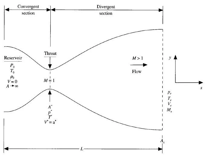
Although the area of the nozzle changes as a function of distance along the nozzle(x - direction). and therefore in reality the flow varies in two-dimensional XY space. But we make the assumption that the flow properties vary only with x. Such flow is defined as quasi-one-dimensional flow.
The governing continuity, momentum, and energy equations for this flow can be expressed as,
Continuity : `rho_1 V_1 A_1 = rho_2 V_2 A_2`
Momentum : `p_1 A_1 +rho_1 V_1^2 A_1 + intpdA =p_2A_2 + rho_2 V_2^2 A_2`
Energy : `h_1 + V_1^2/2 =h_2 + V_2^2/2`
The Mach number variation through the nozzle is governed exclusively by the area ratio A/A* through the relation
`(A/A^(ast))^2= 1/M^2[2/(gamma +1)(1+ (gamma-1)/2 M^2)]^((gamma+1)/(gamma-1))`
As the cross-sectional area of the nozzle is a function of x. Hence, the Mach number also becomes a function of x. In turn, the variation of pressure, density, and temperature as a function of Mach number ( and hence as a function of Al A*, thus x) is given by,
`p/p_0=(1+(gamma-1)/2 M^2)^(-gamma/(gamma-1))`
`rho/rho_0=(1+(gamma-1)/2M^2)^(-1/(gamma-1)`
`T/T_o=(1+(gamma-1)/2M^2)^-1`
When the governing equations are solved at two different points, across the flow through the nozzle we get
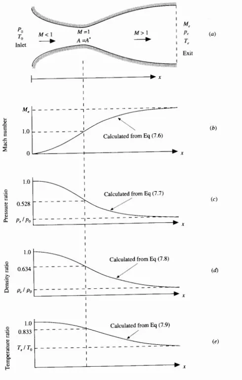
The nozzle flow described above just does not "happen" by itself. As with all mechanical systems, it takes force to accelerate a given mass; the nozzle flow is no different. In this case, the force exerted on the gas to accelerate it through the nozzle is supplied by the pressure ratio across the nozzle, p0 / Pe· For a nozzle with a specified area ratio Ae/A*, the pressure ratio required to establish the subsonic-supersonic isentropic flow must be a very specific value.
-----------------------------------------------------------------------------------------------------------------------------------------------------------
Non-Conservation form :
When the control Volume is moving.
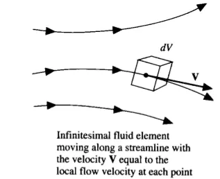
The fundamental physical principles are applied to the fluid inside the control volume. Therefore, instead of looking at the whole flow field at once, with the control volume model we limit our attention to just the fluid in the finite region of the volume itself.
Governing Equations:
As we assume that the flow properties are uniform across any given cross-section of the nozzle. In so doing, we have somewhat twisted the physics of the flow. we would at least like the overall physical principles of (I) mass conservation, (2) Newton's second law, and (3) energy conservation to hold exactly, in spite of our twisted physics due to the quasi-one-dimensional assumption.
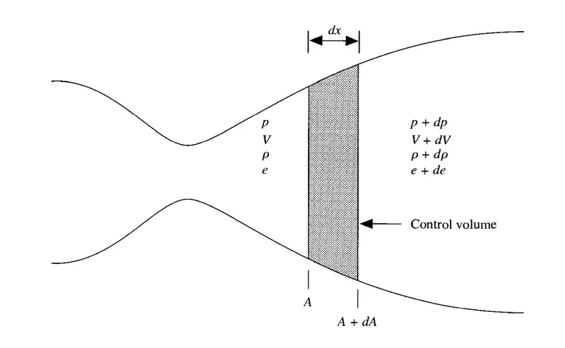
1) mass conservation: The Control volume, which is a slice of the nozzle flow, is taken and the integral form of the continuity equation is applied to it.
`del/(delt)int int int rho dV + int int rho V *dS =0` --> integral form
`(del(rho A))/(delt) + rho A(del V)/(delx)+rho V (delA)/(delx)+VA(delrho)/(delx)=0` ---> continuity equatio`
2) momentum conservation :
`del/(delt) int int int (rho u) dV + int int (rho u V)*dS =-int int(p dS)_x`---> integral form
`rho (delV)/(delt) + rho V (delV)/(delx) = -R(rho(delT)/(delx) +T (delrho)/(delx))` ----> momentum equation `
3) energy conservation :
`del/(delt) int int int rho (e+V^2/2)dV + int int rho (e+V^2/2)V.dS=-int int (p V).dS` ----> integral form
`rho C_v(delT)/(delt) + rhoVC_v(delT)/(delx)= - rhoRT[(delV)/(delx) + V(del(lnA))/(delx}` ---> energy equation `
At this stage, we could readily proceed to set up our numerical solution. But for nozzle flows, the flow-field variables are frequently
expressed in terms of nondimensional variables, where the flow variables are referenced to their reservoir values. The
non-dimensional variables p/p0, rho/rho0, and T/T0 vary between O and I, which is an "aesthetic" advantage when presenting the results.
After non-dimensionalizing the variables the equations come out to be :
`(delrho' )/(delt') = -rho' (delV')/(delx') - rho'V' (del(ln A'))/(delx')-V'(delrho')/(delx')` ---> continuity equation
`(delV')/(delt')=-V'(delV')/(delx')-1/gamma((delT')/(delx')+(T')/(rho')(delrho')/(delx'))` ----> momentum equation
`(delT')/(delt')=-V' (delT')/(delx')-(gamma-1)T'[(delV')/(delx')+V'(del(lnA'))/(delx')]`----> energy equation
Numerical discretization :
The setting up of the finite-difference expressions of the above governing equations is done using MacCormack's explicit technique. To implement a finite-difference solution, we divide the x-axis along the nozzle into a number of discrete grid points as shown below.
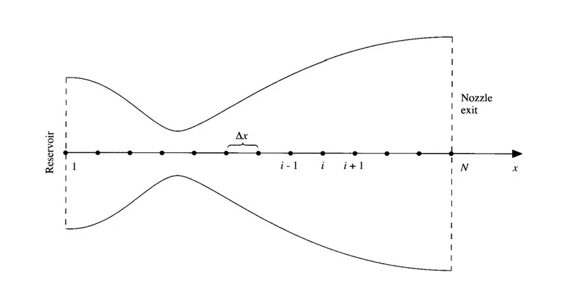
MacCormack's technique is a predictor-corrector method, the Maccormack method is also an explicit finite-difference technique that is second-order-accurate in both space and time. In this time-marching approach, the flow-field variables at time t are known, and we use the difference equations to solve explicitly for the variables at time t + dt.
step-1: Predictor step
A forward differencing scheme is used to calculate the flow variables across the nozzle(spatial derivatives).
`((delrho)/(delt))_i^t= -rho_i^t(V_(i+1)^t-V_i^t)/(Deltax)-rho_i^t V_i^t (lnA_(i+1)-lnA_i)/(Deltax)-V_i^t(rho_(i+1)^t-rho_i^t)/(Deltax)`
Similar to this, the other governing equations are discretized.
step-2: predictor update
we obtain predicted values of rho, v, and T denoted by a bar.
`rho_i^(t+Deltat)= rho_i^t+((delp)/(delt))_i^t Deltat`
Analogous to this, the other variables are updated.
step-3: Corrector step
In the corrector step, we first obtain a predicted value of the time derivative at time t + dt, `((delp)/(delt))_i^(t+Deltat` by substituting the predicted values of p, u, and v into the right side of the continuity equation, replacing the spatial derivatives with rearward differences.
`((delp^bar)/(delt))_i^(t+Deltat)=-rho _i^(t+Deltat) (V_i^(t+Deltat)-V_(i-1)^(t+Deltat))/(Deltax)-rho _i^(t+Deltat) V _i^(t+Deltat) (lnA_i-lnA_(i-1))/(Deltax)-V _i^(t+Deltat) (rho_i^(t+Deltat)-rho_(i-1)^(t+Deltat))/(Deltax)`
step-4: Averaging the predictor derivative and corrector derivative
`((delp)/(delt))_(avg)=0.5[((delp)/(delt))_(pred)+((delp)/(delt))_(c o rrect o r)]`
The value of `((delp)/(delt))_(avg)` is calculated so as to preserve second-order accuracy without the need to calculate values of the second time derivative`((del^2p)/(delt^2))_i^t`, which involves a lot of algebra.
step-5: Final update
`rho_i^(t+Deltat)= rho_i^t+((delp)/(delt))_(avg)*Deltat`
Time step:
The governing system of equations is hyperbolic with respect to time. The stability of the numerical scheme depends upon the CFL number i.e,`CFL = (a+V)(Deltat)/(Deltax)`
where a- speed of sound; V- velocity of the flow(at a node); dt- time step size; dx-grid size
For linear hyperbolic equations, the previous literature says that, for a stable solution CFL<=1. This equation simply states that dt must be less than, or at best equal to, the time it takes a sound wave to move from one grid point to the next.
At a time t, as we go across the domain, the velocity value changes, the speed of sound changes as well, and the grid size is constant. So, to maintain the CFL<=1 , the remaining factor which can be changed is the size of the time step(dt). Therefore, the size of the time-step is calculated at every node of the domain and the minimum value of the time step is chosen for that particular time step.
`Deltat=min(Deltat_1^t,Deltat_2^t,Deltat_3^t,...,Deltat_n^t)`
Boundary Conditions:
An important aspect, because without the physically proper implementation of boundary conditions and their numencally proper
representation, we have no hope whatsoever in obtaining a proper numerical solution to our flow problem.The grid pomts 1 and N represent the two boundary points on the x axis. Point l is essentially in the reservoir; 1t represents an inflow boundary, with flow coming from the reservoir and entering the nozzle. In contrast, point N is an outflow boundary, with flow leaving the nozzle at the nozzle exit. Moreover, the flow velocity at point l is a vey low, subsonic value.
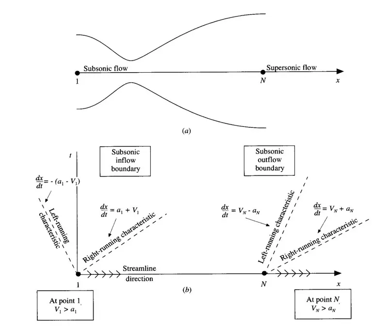
The boundary conditions can be obtained by the method of characteristics(depends on the information transfer). For one-dimensional unsteady flow there exists two real characteristic lines through any point in the xt plane as shown above.Physically, these two characteristics represent infinitely weak Mach waves which are propagating upstream and downstream, respectively.At the subonic inflow boundary, we must fix the values of two dependent flow-field variables and allow one to float, whereas at the supersonic boundary,the value of three variables must be allowed to float.
Inlet BCs: Outlet BCs:
`V_1= 2V_2 -V_3` `V_n=2V_(n-1)-V_(n-2)`
`rho_1=1` `rho_n=2rho_(n-1)-rho_(n-2)`
`T_1=1` `T_n=2T_(n-1)-T_(n-2)`
Initial Conditions:
The closer the initial conditions are to the final steady-state answer, the faster the time-marching procedure will converge, and hence the shorter will be the computer execution time.
`rho= 1-0.3146x`
`T=1-0.2314x`
`V=(0.1+1.09x)T^(1/2)`
`A=1+2.2(x-1.5)^2` `0<=x<=3`
-----------------------------------------------------------------------------------------------------------------------------------------------------------
Conservation form :
When the control Volume is stationary/fixed.
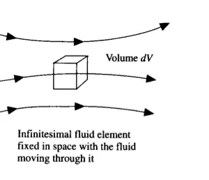
The fundamental physical principles are applied to the fluid inside the control volume and to the fluid crossing the control surface (as the control volume is fixed in space).
Governing equations:
The non-dimensional form of the governing equations:
1) continuity equation : `(del(rho' A'))/(delt)+ (del(rho'A'V'))/(delx')=0`
2) momentum equation : `(del(rho' A' V'))/(delt)+(del[rho' A' V'^2 +(1/gamma)p'A'])/(delx')=(1/gamma)p'(delA')/(delx')`
3)energy equation: `(del[rho'((e')/(gamma-1)+gamma/2V'^2)A'])/(delt')+(del[rho'((e')/(gamma-1)+gamma/2V'^2)V'A'+p'A'V'])/(delx')=0`
Instead of solving for the primitive variables p,rho,v ,T etc we solve for the solutions vector U [the flux vector F, and the source terms J appear on the RHS] as follows:
`U_1=rho'A'`
`U_2=rho'A'V'`
`U_3=rho'((e')/(gamma-1)+gamma/2V'^2)A'`
`F_1=rho'A'V'`
`F_2=rho' A' V'^2 +(1/gamma)p'A'`
`F_3=rho'((e')/(gamma-1)+gamma/2V'^2)V'A'+p'A'V'`
`J_2=(1/gamma)p'(delA')/(delx')`
With these elements, the above governing equations are expressed as:
`(delU_1)/(delt')=-(delF_1)/(delx')`
`(delU_2)/(delt')=-(delF_2)/(delx')+J_2`
`(delU_3)/(delt')=-(delF_3)/(delx')`
To obtain the primitive variables (p, V, T,p, etc.), we must decode
the elements U1, U2, and U3 as follows.
`rho'=U_1/(A')`
`V'=U_2/U_1`
`T'=e'=(gamma-1)(U_3/U_2-gamma/2V'^2)`
`p'=rho'T'`
Therefore, after we obtain U1, U2, and U3 at each time step from the numerical solution, we can immediately calculate the corresponding primitive variables at each time step, rho', V', T', and p',
"PURE" FORM OF THE FLUX TERMS
The flux vector elements F1, F2, and F3 are couched in terms of the primitive variables. Previous literature suggests that when the computer program is written with F 1, F2 , and F3 expressed directly in terms of p', V', p', and e', instabilities develop during the course of the time-marching solution. This behavior is an example of a lack of "purity" in the formulation of the governing equations in conservation form. To avoid numerical instabilities F1, F2, and F3 will be expressed as a function of dependent variables U1, U2, and U3.
`F_1=U_2`
`F_2=(U_2^2)/U_1+(gamma-1)/gamma[U_3-gamma/2(U_2^2)/U_1]`
`F_3=gamma(U_2U_3)/U_1-(gamma(gamma-1))/2U_2^3/U_1^2`
The source term is also expressed in terms of U1, U2, and U3
`J_2=(gamma-1)/gamma(U_3-gamma/2(U_2^2)/U_1)(del(lnA'))/(delx')`
Numerical discretization :
Mac cormack technique:
step-1 : Initialize the F vector
`F_1=U_2`
`F_2=(U_2^2)/U_1+(gamma-1)/gamma[U_3-gamma/2(U_2^2)/U_1]`
`F_3=gamma(U_2U_3)/U_1-(gamma(gamma-1))/2U_2^3/U_1^2`
step-2 : predictor step ---> Forward differencing scheme
`((delU_1)/(delt'))_i^t=- ((F_1)_(i+1)-(F_1)_i)/(Deltax'`
Analogous to this, the other two equations are also forward differenced.
step-3 : predictor update
`(U_1)_(i)^(t+dt)=(U_1)_i^t+((delU_1)/(delt'))_i^t Deltat'`
The other terms are also updated.
step-4 : Updating the flux vectors F,rho,t using the relations mentioned in step1
step-5: corrector step ---> Backward differencing scheme
The predicted values of flux vectors are plugged in the below equation and corrector step derivatives are obtained.
`((delU_1)/(delt'))_i^(t+dt)=-((F_1)_i-(F_1)_(i-1))/(delx'`
step-6 : Calculating the average
`(delU_1)/(delt))_(avg)=0.5[((delU_1)/(delt))_(pred)+((delU_1)/(delt))_(c o rrect o r)]`
step-7 : Final update
`(U_1)_i^(t+Deltat)= (U_1)_i^t+((delU_1)/(delt))_(avg)*Deltat`
Boundary Conditions :
The boundary conditions for the subsonic-supersonic isentropic flow solution using the conservation form of the governing equations are theoretically the same as the non-conservation form.At the subonic inflow boundary, we must fix the values of two primitive dependent flow-field variables and allow one to float, whereas at the supersonic boundary,the value of three variables must be allowed to float.As the flow domain, is in terms of solution vectors U,the boundaries are also expressed in terms of U.
Inlet BCs:
`U_(1(i=1) = (rho'A')_(i=1)=A'_(i=1)=fixed value`
`U_(2(i=1))=2U_(2(i=2))-U_(2(i=3))`
`U_3=U_1((T')/(gamma-1)+gamma/2V'^2)`
Outlet BCs:
`(U_1)_n=2(U_1)_(n-1)-(U_1)_(n-2)`
`(U_2)_n=2(U_2)_(n-1)-(U_2)_(n-2)`
`(U_3)_n=2(U_3)_(n-1)-(U_3)_(n-2)`
Initial Conditions:
Since the dependent variables being solved are U1, U2, and U3, we need initial conditions for these same variables at time t = 0 in order to start the finite-difference solution. The initial conditions for U1, U2, and U3 also allow initial conditions for F1,F2, and F3.
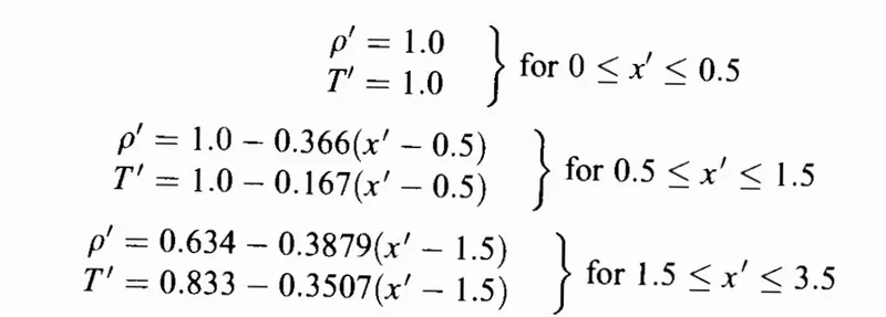
The initial condition for the variation of V' is synthesized by
taking advantage of the fact that one of the dependent variables in our governing equations, namely, U2, is physically the local mass flow; that is, U2 = p'A'V'. Therefore,for the initial conditions only, let us assume a constant mass flow through the nozzle and calculate V' as
`V'=U_2/(rho' A') =0.59/(rho' A')`
The value 0.59 is chosen for U2 because it is close to the exact analytical value of the steady-state mass flow (which for this case is 0.579).Finally, the U1,U2 and U3 are obtained from the relation between the solution vectors and primitive variables rho',A',V'etc.
------------------------------------------------------------------------------------------------------------------------------
Matlab code:
Non-Conservation form:
clear all
close all
clc

% solving the flow through nozzle Qausi 1D using MacCormack method

%creating the flow domain

n=31;
x=linspace(0,3,n);
dx=x(2)-x(1);
gamma=1.4;

%initial profiles of the flow variables

rho=1-0.3146*x;
t=1-0.2314*x;
v=(0.1+1.09*x).*t.^0.5;
a=1+2.2*(x-1.5).^2;

c=0.7;
%time steps
dt1=c*(dx./(v+sqrt(t)));
dt=min(dt1);
nt=1400;

% time marching explicit maccormack method
%time loop

for k=1:nt


    %copy of initial profiles
    rho_old=rho;
    t_old=t;
    v_old=v;

    %space loop

    for i=2:n-1

        %predictor step- forward differencing
        dvdx=(v(i+1)-v(i))/dx;
        drhodx=(rho(i+1)-rho(i))/dx;
        dtdx=(t(i+1)-t(i))/dx;
        dlogadx=(log(a(i+1))-log(a(i)))/dx;

        %continuity equation
        drhodt_p(i) = -rho(i)*dvdx-rho(i)*v(i)*dlogadx-v(i)*drhodx;

        %momentum equation
        dvdt_p(i) = -v(i)*dvdx-(1/gamma)*(dtdx+(t(i)/rho(i))*drhodx);

        %energy equation
        dtdt_p(i) = -v(i)*dtdx-(gamma-1)*t(i)*(dvdx+v(i)*dlogadx);

        %predictor step solution update

        rho(i)=rho(i)+drhodt_p(i)*dt;
        v(i)=v(i)+dvdt_p(i)*dt;
        t(i)=t(i)+dtdt_p(i)*dt;


        %corrector step- backward differencing
        dvdx=(v(i)-v(i-1))/dx;
        drhodx=(rho(i)-rho(i-1))/dx;
        dtdx=(t(i)-t(i-1))/dx;
        dlogadx=(log(a(i))-log(a(i-1)))/dx;

        %continuity equation
        drhodt_c(i) = -rho(i)*dvdx-rho(i)*v(i)*dlogadx-v(i)*drhodx;

        %momentum equation
        dvdt_c(i) = -v(i)*dvdx-(1/gamma)*(dtdx+(t(i)/rho(i))*drhodx);

        %energy equation
        dtdt_c(i) = -v(i)*dtdx-(gamma-1)*t(i)*(dvdx+v(i)*dlogadx);


    end

    %computing the average time derivative

    dvdt=0.5*(dvdt_p+dvdt_c);
    drhodt=0.5*(drhodt_p+drhodt_c);
    dtdt=0.5*(dtdt_p+dtdt_c);

    %final solution update

    for i=2:n-1

        rho(i)=rho_old(i)+drhodt(i)*dt;

        v(i)=v_old(i)+dvdt(i)*dt;

        t(i)=t_old(i)+dtdt(i)*dt;


    end

    % applying boundary conditions

    %inlet
    v(1)=2*v(2)-v(3);

    %outlet
    v(n)=2*v(n-1)-v(n-2);
    rho(n)=2*rho(n-1)-rho(n-2);
    t(n)=2*t(n-1)-t(n-2);


%Mach number
m=v./sqrt(t);

%pressure
p=rho.*t;

%mass flow rate
mv=rho.*a.*v;

throat_val=round(length(x)/2);
v_throat(k)=v(throat_val);
rho_throat(k)=rho(throat_val);
t_throat(k)=t(throat_val);
p_throat(k)=p(throat_val);
m_throat(k)=m(throat_val);

figure(1)
hold on
if k==1
    plot(x,mv,LineWidth=2)
end

if k==50
    plot(x,mv,LineWidth=2)
end

if k==250
    plot(x,mv,LineWidth=2)
end

if k==500
    plot(x,mv,LineWidth=2)
end

if k==800
    plot(x,mv,LineWidth=2)
end

if k==1400
    plot(x,mv,LineWidth=2)
end

end
xlabel("non-dimensional length of the nozzle");
ylabel('Mass flow rate');
legend('1dt','50dt','250dt','500dt','800dt','1400dt');
title('Trasnsient varaiation of mass flow rate');

%plotting

%plotting the steady-state primitive variables

figure(2)
subplot(5,1,1)
plot(x,v);
xlabel('length of the domain');
ylabel('velocity');
text=sprintf('number of time step=%d',k);
title(text);

subplot(5,1,2)
plot(x,p);
xlabel('length of the domain');
ylabel('pressure');
text=sprintf('number of time step=%d',k);
title(text);


subplot(5,1,3)
plot(x,rho);
xlabel('length of the domain');
ylabel('density');
text=sprintf('number of time step=%d',k);
title(text);

 subplot(5,1,4)
plot(x,t);
xlabel('length of the domain');
ylabel('temperature');
text=sprintf('number of time step=%d',k);
title(text);

subplot(5,1,5)
plot(x,m);
xlabel('length of the domain');
ylabel('Mach Number');
text=sprintf('number of time step=%d',k);
title(text);

figure(3)
%plotting mass flow rate across the length of the nozzle
plot(x,mv);
xlabel("length of the nozzle");
ylabel('mass flow rate')

%plotting the variation of primitive variables at throat wrt time

figure(4)
subplot(5,1,1)
plot(v_throat);
xlabel('time step');
ylabel('velocity');
title('transient variation of primitive variables at throat');

subplot(5,1,2)
plot(p_throat);
xlabel('time step');
ylabel('pressure');

subplot(5,1,3)
plot(rho_throat);
xlabel('time step');
ylabel('density');


subplot(5,1,4)
plot(t_throat);
xlabel('time step');
ylabel('temperature');


subplot(5,1,5)
plot(m_throat);
xlabel('time step');
ylabel('Mach number');
Explanation of the code:
1. First, the domain is created and the initial arrays for rho,temperature,velocity,area are calculated.
2. Constants such as CFL number, gamma are specified.
3. The time-step is calculated taking into account the CFL criterion.
4. First, a time loop is created.So,at each and every time step, we calculate the primitive variables by solving the non-conservative form of governing equations using the forward differencing scheme-predictor step for the whole domain(space loop).Then these values are updated.
5.Similarly, this process is repeated for the corrector step.
6. Average is calculated using the values obtained from both the predictor and corrector steps.
7. Final updation of the primitive variables is done.Then the boundary conditions are applied i,e from the second time-step the boundary conditions will be incorporated in the domain.
8.The flow parameters at the throat are calculated.
9. Then we plot the flow parameters such as velocity,pressure,temperature,Mach number,rho at the last time-step, also the flow parameters at the throat at different time steps are plotted.
10. Mass flow rate is calculated and plotted,also mass flow rate at different time steps are plotted.
conservative code:
clear all
close all
clc

% solving the flow through nozzle Qausi 1D using MacCormack method

%creating the flow domain

n=31;
x=linspace(0,3,n);
dx=x(2)-x(1);
gamma=1.4;

%initial profiles of the flow variables

for i=1:n
    if x(i)<=0.5 && x(i)>=0
        rho(i)=1;
        t(i)=1;
    end

    if x(i)<=1.5 && x(i)>=0.5
        rho(i)= 1-0.366*(x(i)-0.5);
        t(i)=1-0.167*(x(i)-0.5);
    end

    if x(i)>=1.5 && x(i)<=3.5
        rho(i)=0.634-0.3879*(x(i)-1.5);
        t(i)=0.833-0.3507*(x(i)-1.5);
    end
end

a=1+2.2*(x-1.5).^2;  % crossectional area

%initialising the vector field

v=0.59./(rho.*a);

%initialising the solution vectors u1,u2 and u3

u1=rho.*a;
u2=rho.*a.*v;
u3=rho.*(t./(gamma-1)+(gamma/2).*v.^2).*a;

%            f1=u2;
%         f2=(u2.^2)./(u1)+(gamma-1)/(gamma).*(u3-(gamma/2).*(u2.^2)./(u1));
%         f3=gamma.*(u2.*u3)./u1-(gamma*(gamma-1))/2.*(u2.^3)./(u1.^2);
%

c=0.5;    % courant number


nt=1400;
%time steps
dt1=c*(dx./(v+sqrt(t)));
dt=min(dt1);


% time marching explicit maccormack method
%time loop

for k=1:nt
    %updating from the previous time step
    f1=u2;
    f2=(u2.^2)./(u1)+(gamma-1)/(gamma).*(u3-(gamma/2).*(u2.^2)./(u1));
    f3=gamma.*(u2.*u3)./u1-(gamma*(gamma-1))/2.*(u2.^3)./(u1.^2);

    %     %time steps
    %     dt1=c*(dx./(v+sqrt(t)));
    %     dt=min(dt1);


    %copy of initial profiles
    u1_old=u1;
    u2_old=u2;
    u3_old=u3;

    %space loop

    for i=2:n-1

        %predictor step- forward differencing

        %continuity equation
        du1dt_p(i) = - (f1(i+1)-f1(i))/dx;

        j2=(1/gamma)*rho(i)*t(i)*(a(i+1)-a(i))/dx;
        %momentum equation
        du2dt_p(i)=- ((f2(i+1)-f2(i)))/dx + j2;

        %energy equation
        du3dt_p(i) = - (f3(i+1)-f3(i))/dx;

        %predictor step solution update

        u1(i)=u1(i)+du1dt_p(i)*dt;
        u2(i)=u2(i)+du2dt_p(i)*dt;
        u3(i)=u3(i)+du3dt_p(i)*dt;

        % updation of flux terms(as they will be reqd on rhs of corr step)


    end
    f1=u2;
    f2=(u2.^2)./(u1)+(gamma-1)/(gamma).*(u3-(gamma/2).*(u2.^2)./(u1));
    f3=gamma.*(u2.*u3)./u1-(gamma*(gamma-1))/2.*(u2.^3)./(u1.^2);
    rho=u1./a;
    t=(gamma-1)*((u3)./(u1)-(gamma/2)*(u2./u1).^2)
    %% corrector step

    for i=2:n-1

        du1dt_c(i)= - (f1(i)-f1(i-1))/dx;

        j2=(1/gamma)*rho(i)*t(i)*(a(i)-a(i-1))/dx;
        du2dt_c(i)= - (f2(i)-f2(i-1))/dx+j2;

        du3dt_c(i)= - (f3(i)-f3(i-1))/dx;


    end


    %     end

    %computing the average time derivative

    du1dt=0.5*(du1dt_p+du1dt_c);
    du2dt=0.5*(du2dt_p+du2dt_c);
    du3dt=0.5*(du3dt_p+du3dt_c);

    %final solution update

    for i=2:n-1

        u1(i)=u1_old(i)+du1dt(i)*dt;
        u2(i)=u2_old(i)+du2dt(i)*dt;
        u3(i)=u3_old(i)+du3dt(i)*dt;


    end

    % applying boundary conditions

    %inlet
    u1(1)=rho(1)*a(1);
    u2(1)=2*u2(2)-u2(3);
    u3(1)=u1(1)*(t(1)/(gamma-1)+(gamma/2)*v(1)^2);

    %outlet
    u1(n)=2*u1(n-1)-u1(n-2);
    u2(n)=2*u2(n-1)-u2(n-2);
    u3(n)=2*u3(n-1)-u3(n-2);

    % finding out the primitive variables

    v=u2./u1;
    p=rho.*t
    rho=u1./a;
    t=(gamma-1)*((u3)./(u1)-(gamma/2)*(u2./u1).^2)

    %Mach number
    m=v./sqrt(t);

    %pressure
    p=rho.*t;

    %mass flow rate
    mv=rho.*a.*v;

    throat_val=round(length(x)/2);
    v_throat(k)=v(throat_val);
    rho_throat(k)=rho(throat_val);
    t_throat(k)=t(throat_val);
    p_throat(k)=p(throat_val);
    m_throat(k)=m(throat_val);

    figure(1)
    hold on
    if k==1
        plot(x,mv,LineWidth=2)
    end

    if k==50
        plot(x,mv,LineWidth=2)
    end

    if k==250
        plot(x,mv,LineWidth=2)
    end

    if k==500
        plot(x,mv,LineWidth=2)
    end

    if k==800
        plot(x,mv,LineWidth=2)
    end

    if k==1400
        plot(x,mv,LineWidth=2)
    end

end

xlabel("non-dimensional length of the nozzle");
ylabel('Mass flow rate');
legend('1dt','50dt','250dt','500dt','800dt','1400dt');
title('Trasnsient varaiation of mass flow rate');

%plotting

%plotting the steady-state primitive variables

figure(2)
subplot(5,1,1)
plot(x,v);
xlabel('length of the domain');
ylabel('velocity');
text=sprintf('number of time step=%d',k);
title(text);

subplot(5,1,2)
plot(x,p);
xlabel('length of the domain');
ylabel('pressure');
text=sprintf('number of time step=%d',k);
title(text);


subplot(5,1,3)
plot(x,rho);
xlabel('length of the domain');
ylabel('density');
text=sprintf('number of time step=%d',k);
title(text);

subplot(5,1,4)
plot(x,t);
xlabel('length of the domain');
ylabel('temperature');
text=sprintf('number of time step=%d',k);
title(text);

subplot(5,1,5)
plot(x,m);
xlabel('length of the domain');
ylabel('Mach Number');
text=sprintf('number of time step=%d',k);
title(text);

figure(3)
%plotting mass flow rate across the length of the nozzle
plot(x,mv);
xlabel("length of the nozzle");
ylabel('mass flow rate');

%plotting the variation of primitive variables at throat wrt time

figure(4)
subplot(5,1,1)
plot(v_throat);
xlabel('time step');
ylabel('velocity');
title('transient variation of primitive variables at throat');

subplot(5,1,2)
plot(p_throat);
xlabel('time step');
ylabel('pressure');

subplot(5,1,3)
plot(rho_throat);
xlabel('time step');
ylabel('density');


subplot(5,1,4)
plot(t_throat);
xlabel('time step');
ylabel('temperature');


subplot(5,1,5)
plot(m_throat);
xlabel('time step');
ylabel('Mach number');
Explanation of the code:
1. First, the domain is created and the initial arrays for rho,temperature are calculated using if cmd,as the values vary along different sections of x.Then the area,initial velocity array,u1,u2,u3,f1,f2and f3 are calculated.
2. Constants such as CFL number, gamma are specified.
3. The time-step is calculated taking into account the CFL criterion.
4. First, a time loop is created.So,at each and every time step, we calculate the solution variables by solving the conservative form of the governing equations which are interms of U,F and J using the forward differencing scheme-predictor step for the whole domain(space loop).Then these values are updated.As the u values are updated f,j,rho and t values should be updated updated as well.
5.Similarly, this process is repeated for the corrector step.
6. Average is calculated using the values obtained from both the predictor and corrector steps.
7. Final updation of the solution variables is done.Then the boundary conditions are applied i,e from the second time-step the boundary conditions will be incorporated in the domain.
8.After getting the final value of solution variables, the primitive variables are found out.Then the flow parameters at the throat are calculated as well.
9. Then we plot the flow parameters such as velocity,pressure,temperature,Mach number,rho at the last time-step, also the flow parameters at the throat at different time steps are plotted.
10. Mass flow rate is calculated and plotted,also mass flow rate at different time steps is plotted.
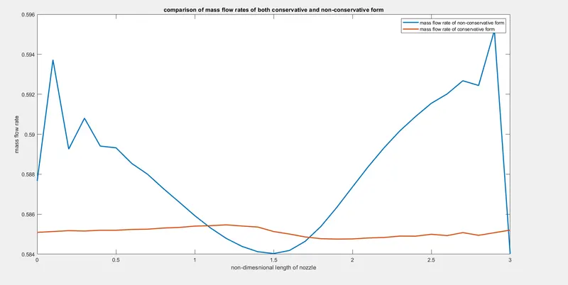
To get the mass flow rates of both conservative and non-conservative forms in a single plot,the above codes are converted into functions which takes inputs (n,x,dx,gamma,nt) and calculates the mass flow rate.
Main function code:
clear all
close all
clc

% solving the flow through nozzle Qausi 1D using MacCormack method

%creating the flow domain

n=31;
x=linspace(0,3,n);
dx=x(2)-x(1);
gamma=1.4;
nt=1400;


[mv_c]=test1(n,dx,gamma,nt,x);
[mv_nc]=test2(n,dx,gamma,nt,x);

figure(5)
plot(x,mv_nc,x,mv_c,LineWidth=2)
function code:
non-conservative form:
function [mv_c]=test1(n,dx,gamma,nt,x)
%initial profiles of the flow variables

for i=1:n
    if x(i)<=0.5 && x(i)>=0
        rho(i)=1;
        t(i)=1;
    end

    if x(i)<=1.5 && x(i)>=0.5
        rho(i)= 1-0.366*(x(i)-0.5);
        t(i)=1-0.167*(x(i)-0.5);
    end

    if x(i)>=1.5 && x(i)<=3.5
        rho(i)=0.634-0.3879*(x(i)-1.5);
        t(i)=0.833-0.3507*(x(i)-1.5);
    end
end

a=1+2.2*(x-1.5).^2;  % crossectional area

%initialising the vector field

v=0.59./(rho.*a);

%initialising the solution vectors u1,u2 and u3

u1=rho.*a;
u2=rho.*a.*v;
u3=rho.*(t./(gamma-1)+(gamma/2).*v.^2).*a;

%            f1=u2;
%         f2=(u2.^2)./(u1)+(gamma-1)/(gamma).*(u3-(gamma/2).*(u2.^2)./(u1));
%         f3=gamma.*(u2.*u3)./u1-(gamma*(gamma-1))/2.*(u2.^3)./(u1.^2);
%

c=0.5;    % courant number


%time steps
dt1=c*(dx./(v+sqrt(t)));
dt=min(dt1);


% time marching explicit maccormack method
%time loop

for k=1:nt
    %updating from the previous time step
    f1=u2;
    f2=(u2.^2)./(u1)+(gamma-1)/(gamma).*(u3-(gamma/2).*(u2.^2)./(u1));
    f3=gamma.*(u2.*u3)./u1-(gamma*(gamma-1))/2.*(u2.^3)./(u1.^2);

    %     %time steps
    %     dt1=c*(dx./(v+sqrt(t)));
    %     dt=min(dt1);


    %copy of initial profiles
    u1_old=u1;
    u2_old=u2;
    u3_old=u3;

    %space loop

    for i=2:n-1

        %predictor step- forward differencing

        %continuity equation
        du1dt_p(i) = - (f1(i+1)-f1(i))/dx;

        j2=(1/gamma)*rho(i)*t(i)*(a(i+1)-a(i))/dx;
        %momentum equation
        du2dt_p(i)=- ((f2(i+1)-f2(i)))/dx + j2;

        %energy equation
        du3dt_p(i) = - (f3(i+1)-f3(i))/dx;

        %predictor step solution update

        u1(i)=u1(i)+du1dt_p(i)*dt;
        u2(i)=u2(i)+du2dt_p(i)*dt;
        u3(i)=u3(i)+du3dt_p(i)*dt;

        % updation of flux terms(as they will be reqd on rhs of corr step)


    end
    f1=u2;
    f2=(u2.^2)./(u1)+(gamma-1)/(gamma).*(u3-(gamma/2).*(u2.^2)./(u1));
    f3=gamma.*(u2.*u3)./u1-(gamma*(gamma-1))/2.*(u2.^3)./(u1.^2);
    rho=u1./a;
    t=(gamma-1)*((u3)./(u1)-(gamma/2)*(u2./u1).^2)
    %% corrector step

    for i=2:n-1

        du1dt_c(i)= - (f1(i)-f1(i-1))/dx;

        j2=(1/gamma)*rho(i)*t(i)*(a(i)-a(i-1))/dx;
        du2dt_c(i)= - (f2(i)-f2(i-1))/dx+j2;

        du3dt_c(i)= - (f3(i)-f3(i-1))/dx;


    end


    %     end

    %computing the average time derivative

    du1dt=0.5*(du1dt_p+du1dt_c);
    du2dt=0.5*(du2dt_p+du2dt_c);
    du3dt=0.5*(du3dt_p+du3dt_c);

    %final solution update

    for i=2:n-1

        u1(i)=u1_old(i)+du1dt(i)*dt;
        u2(i)=u2_old(i)+du2dt(i)*dt;
        u3(i)=u3_old(i)+du3dt(i)*dt;


    end

    % applying boundary conditions

    %inlet
    u1(1)=rho(1)*a(1);
    u2(1)=2*u2(2)-u2(3);
    u3(1)=u1(1)*(t(1)/(gamma-1)+(gamma/2)*v(1)^2);

    %outlet
    u1(n)=2*u1(n-1)-u1(n-2);
    u2(n)=2*u2(n-1)-u2(n-2);
    u3(n)=2*u3(n-1)-u3(n-2);

    % finding out the primitive variables

    v=u2./u1;
    p=rho.*t
    rho=u1./a;
    t=(gamma-1)*((u3)./(u1)-(gamma/2)*(u2./u1).^2)

    %Mach number
    m=v./sqrt(t);

    %pressure
    p=rho.*t;

    %mass flow rate
    mv_c=rho.*a.*v;

end
conservative form:
function [mv_nc]=test2(n,dx,gamma,nt,x)

%initial profiles of the flow variables

rho=1-0.3146*x;
t=1-0.2314*x;
v=(0.1+1.09*x).*t.^0.5;
a=1+2.2*(x-1.5).^2;

c=0.7;
%time steps
dt1=c*(dx./(v+sqrt(t)));
dt=min(dt1);
nt=1400;

% time marching explicit maccormack method
%time loop

for k=1:nt


    %copy of initial profiles
    rho_old=rho;
    t_old=t;
    v_old=v;

    %space loop

    for i=2:n-1

        %predictor step- forward differencing
        dvdx=(v(i+1)-v(i))/dx;
        drhodx=(rho(i+1)-rho(i))/dx;
        dtdx=(t(i+1)-t(i))/dx;
        dlogadx=(log(a(i+1))-log(a(i)))/dx;

        %continuity equation
        drhodt_p(i) = -rho(i)*dvdx-rho(i)*v(i)*dlogadx-v(i)*drhodx;

        %momentum equation
        dvdt_p(i) = -v(i)*dvdx-(1/gamma)*(dtdx+(t(i)/rho(i))*drhodx);

        %energy equation
        dtdt_p(i) = -v(i)*dtdx-(gamma-1)*t(i)*(dvdx+v(i)*dlogadx);

        %predictor step solution update

        rho(i)=rho(i)+drhodt_p(i)*dt;
        v(i)=v(i)+dvdt_p(i)*dt;
        t(i)=t(i)+dtdt_p(i)*dt;


        %corrector step- backward differencing
        dvdx=(v(i)-v(i-1))/dx;
        drhodx=(rho(i)-rho(i-1))/dx;
        dtdx=(t(i)-t(i-1))/dx;
        dlogadx=(log(a(i))-log(a(i-1)))/dx;

        %continuity equation
        drhodt_c(i) = -rho(i)*dvdx-rho(i)*v(i)*dlogadx-v(i)*drhodx;

        %momentum equation
        dvdt_c(i) = -v(i)*dvdx-(1/gamma)*(dtdx+(t(i)/rho(i))*drhodx);

        %energy equation
        dtdt_c(i) = -v(i)*dtdx-(gamma-1)*t(i)*(dvdx+v(i)*dlogadx);


    end

    %computing the average time derivative

    dvdt=0.5*(dvdt_p+dvdt_c);
    drhodt=0.5*(drhodt_p+drhodt_c);
    dtdt=0.5*(dtdt_p+dtdt_c);

    %final solution update

    for i=2:n-1

        rho(i)=rho_old(i)+drhodt(i)*dt;

        v(i)=v_old(i)+dvdt(i)*dt;

        t(i)=t_old(i)+dtdt(i)*dt;


    end

    % applying boundary conditions

    %inlet
    v(1)=2*v(2)-v(3);

    %outlet
    v(n)=2*v(n-1)-v(n-2);
    rho(n)=2*rho(n-1)-rho(n-2);
    t(n)=2*t(n-1)-t(n-2);


%Mach number
m=v./sqrt(t);

%pressure
p=rho.*t;

%mass flow rate
mv_nc=rho.*a.*v;

end
Results :
steady-state primitive variables
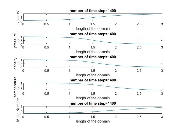
Non-conservative form
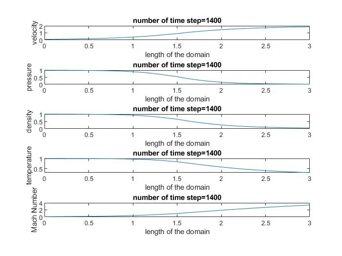
conservative form
Transient variation of primitive variables at the throat:
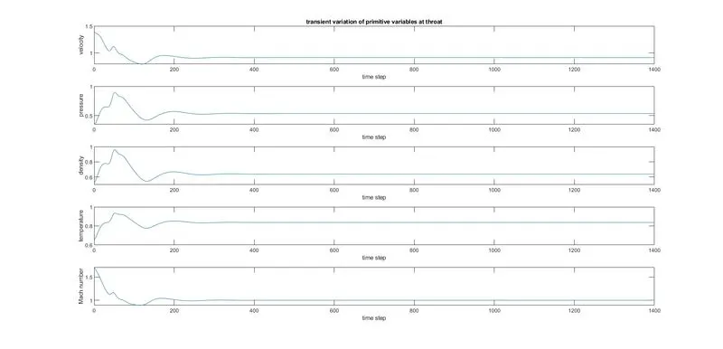
Non-conservative form
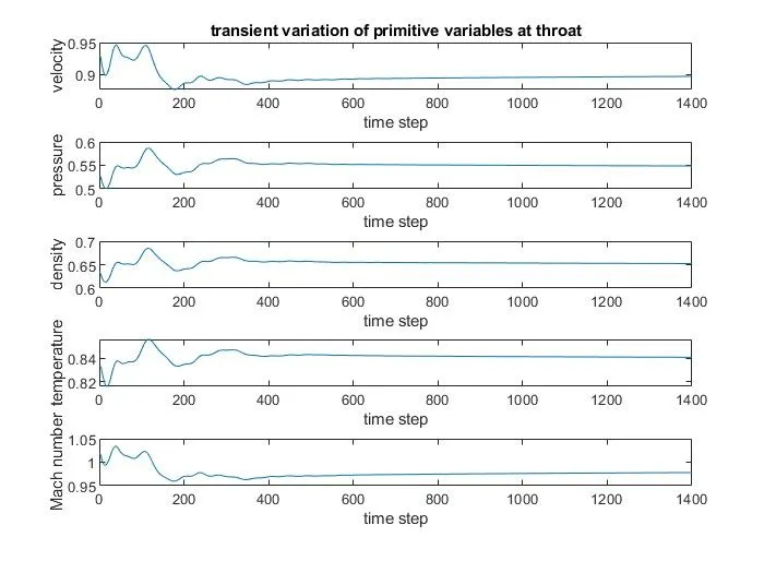
conservative form
Mass flow rates at different time steps:
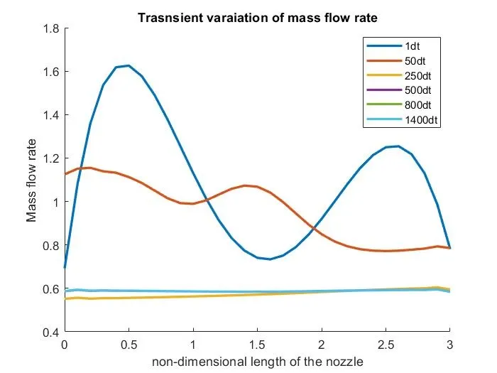
Non-conservative form
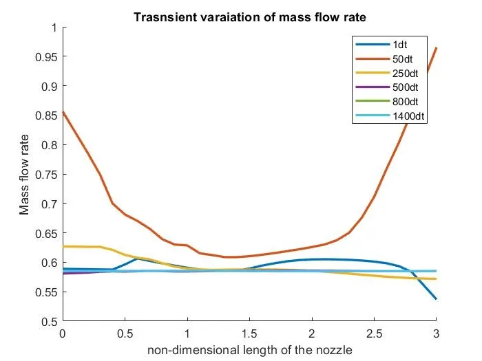
conservative form
Normalised mass flow rate :
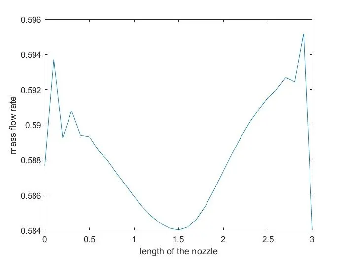
Non-conservative form
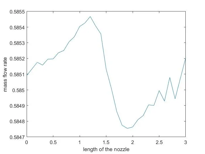
comparison of mass flow rates :
Grid-independent test:
| rho | pressure | temp | Mach | rho error | p error | t error | ||
| non-conservative 31 | 0.639059 | 0.534637 | 0.8366 | 0.999161 | 0.00792 | 0.01241 | 0.0043 | |
| 61 pts | 0.637515 | 0.532548 | 0.835349 | 0.999765 | 0.00551 | 0.00854 | 0.00281 | |
| cons 31 pts | 0.65238 | 0.5487 | 0.841075 | 0.977993 | 0.02817 | 0.03773 | 0.0096 | |
| conservative 61pts | 0.63899 | 0.533977 | 0.835658 | 0.997835 | 0.00781 | 0.01119 | 0.00318 | |
| exact analytical values | 0.634 | 0.528 | 0.833 | 1 | ||||
Observations and Conclusion:
1. The non-conservative form leads to smaller errors compared to the conservative form.
2. The conservation form yields a constant mass flow rate compared to the non-conservation form.
3.Comparing the amount of computational effort to achieve a solution, the conservation form requires more work as the equation is getting decomposed.