Week 6 - CHT Analysis on a Graphics card
Aim :
To perform steady-state conjugate heat transfer analysis on a hypothetical graphics card.
Introduction :
A graphics card is an expansion card that generates a feed of output images to a display device (such as a computer monitor). At the core is the graphics processing unit (GPU), which is the main component that performs computations. As the processing power of graphics cards has increased, so has their demand for electrical power. Current high-performance graphics cards tend to consume large amounts of power. While CPU and power supply makers have recently moved toward higher efficiency, power demands of GPUs have continued to rise, so graphics cards may have the largest power consumption of any individual part of a computer. Modern graphics cards usually require a power consumption of over 75 watts. Providing adequate cooling becomes a challenge in such computers.
To enhance the heat transfer, a heat sink is mounted on the graphics card. A heat sink spreads out the heat produced by the graphics processing unit evenly throughout the heat sink and unit itself. The heat sink commonly has a fan mounted as well to cool the heat sink and the graphics processing unit. Not all cards have heat sinks, for example, some cards are liquid-cooled and instead have a water block; additionally, cards from the 1980s and early 1990s did not produce much heat, and did not require heatsinks. Most modern graphics cards need a proper thermal solution. If the hot spots are not analyzed and taken care of properly it leads to overheating, and the chip will trigger a thermal shutdown.
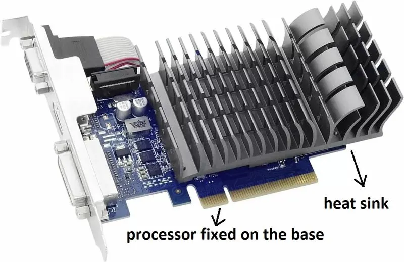
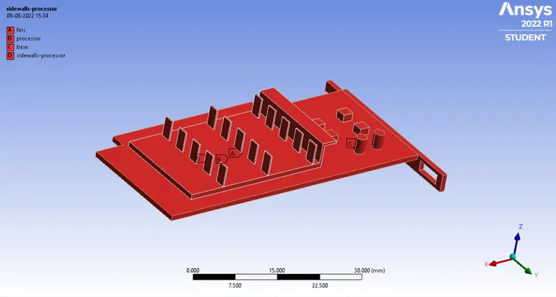
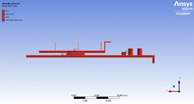
In this case, conjugate heat transfer analysis is performed on a scaled-down model of a hypothetical graphics card which consists of all the main components of an actual graphics card.
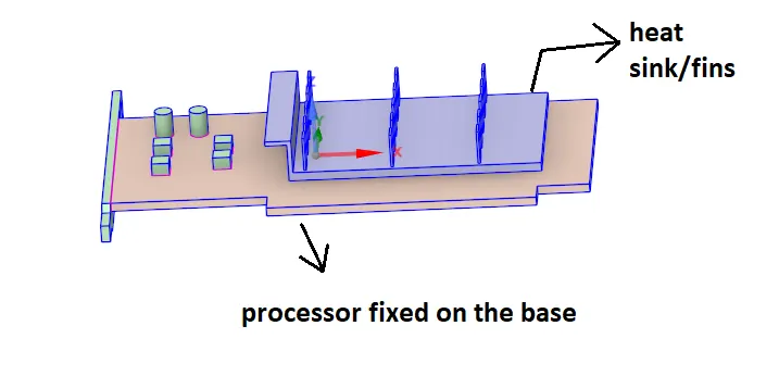
model of a graphics card
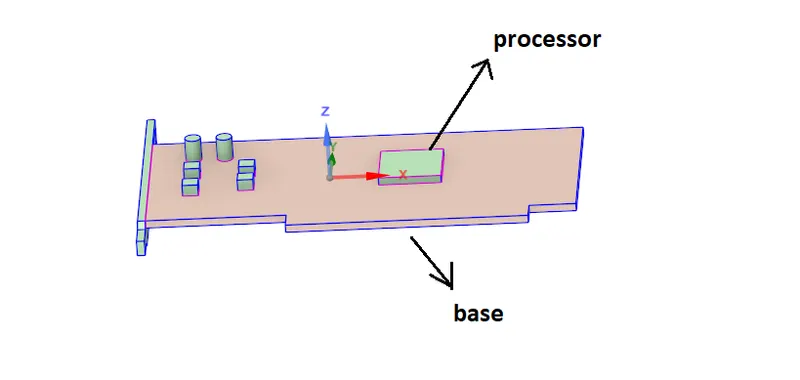
model of graphics card without a heat sink
Conjugate heat transfer corresponds with the combination of heat transfer in solids and heat transfer in fluids. In solids, conduction often dominates whereas, in fluids, convection usually dominates. Conjugate heat transfer is observed in many situations. For example, heat sinks are optimized to combine heat transfer by conduction in the heat sink with the convection in the surrounding fluid.
In any CFD analysis, the workflow that is followed is
Setting up the geometry ----> Meshing ----> setting up the solver ---->solving ---->post-processing results
step-1 Setting up the geometry :
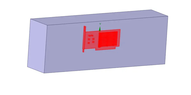
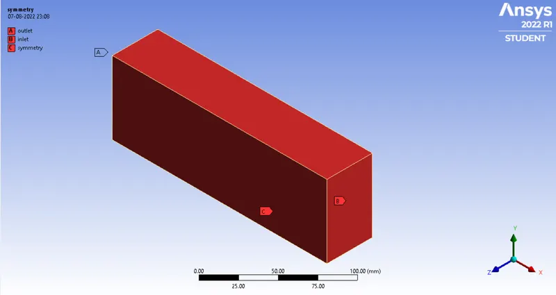
First, the pre-designed 3D geometry of the graphics card is imported to the Spaceclaim module to create an enclosure around the graphics card.
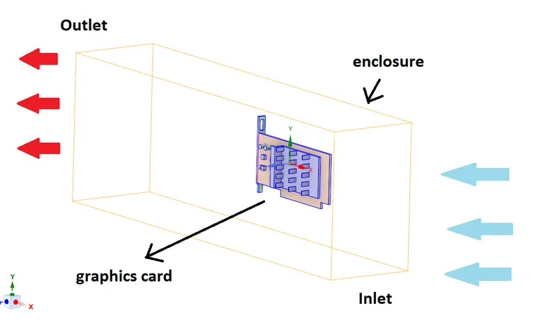
Then, the share feature is used for sharing the common interfaces between the graphics card and the fluid volume so that the information transfer takes place properly.
common interface sharing
Then we can proceed further to meshing the geometry.
step-2 Creating the mesh:
case-1 Baseline mesh :
An automated mesh is generated with tetrahedrons as the major elements consisting of 82129 elements and 15488 nodes.
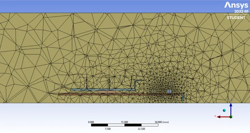
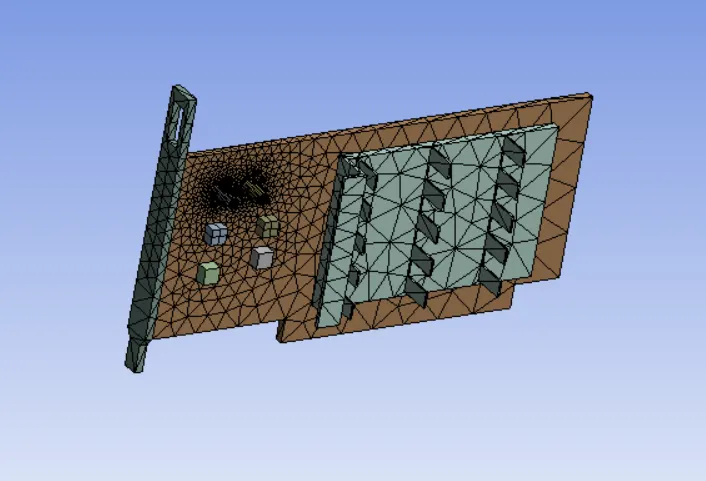
Then the quality of the mesh is checked using the mesh metric in mesh settings, which shows that most of the elements fall above 0.8(1 being the perfect element) and the least elements fall below 0.13, which is perfectly fine for a base mesh.
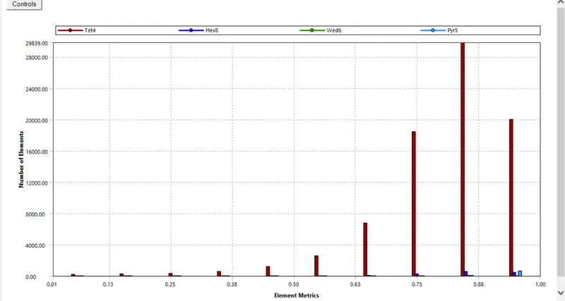
Then the naming of the components and faces is done accordingly.
case-2 mesh refinement
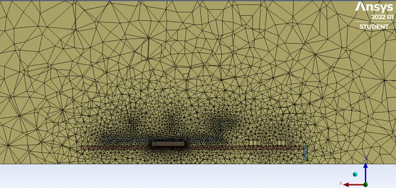
As we are interested to calculate the heat transfer coefficient values at the base, processor, and fins. So we decrease the mesh size in the following regions to get accurate results.
Mesh --> Insert method --> body sizing --> select body --> element size --> generate
fins element size - 0.5mm, processor element size- 0.25mm , 445309 elements & 80400 nodes
step-3 Setting up the solver in Ansys Fluent:
In this step, we define various parameters like initial and boundary conditions, materials used, time steps(for transient), turbulence model, etc which captures the physics to be simulated.
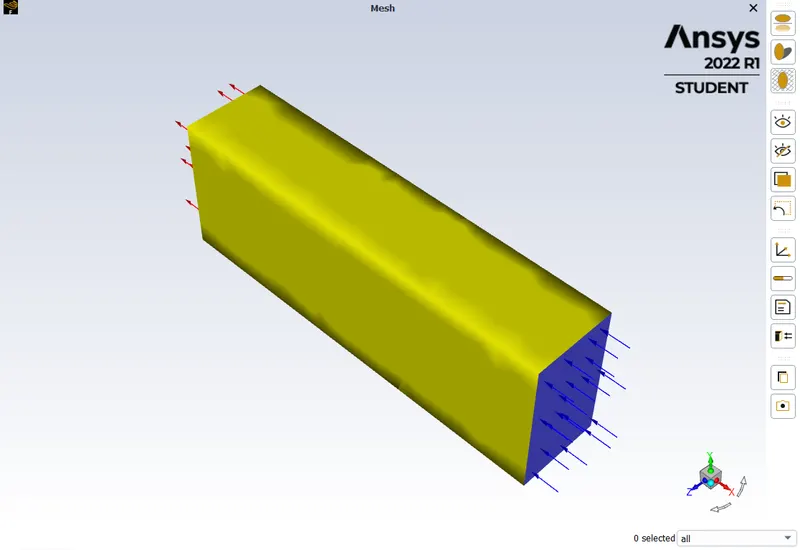
First, we set up the physics by choosing the pressure-based solver which was particularly designed for low-speed incompressible flows(low Mach number), while the density-based solver was mainly designed for high-speed compressible flows(high Mach number).
Then, the steady-state solver is checked, as we are interested in seeing the final results after the flow variables become steady. Along with the standard governing PDEs, we will also be solving the Energy equation.
The turbulence model is selected as the k-epsilon model i.e, the standard k-epsilon model with standard wall function, which solves for turbulence kinetic energy 'k' and its dissipation rate 'epsilon'.
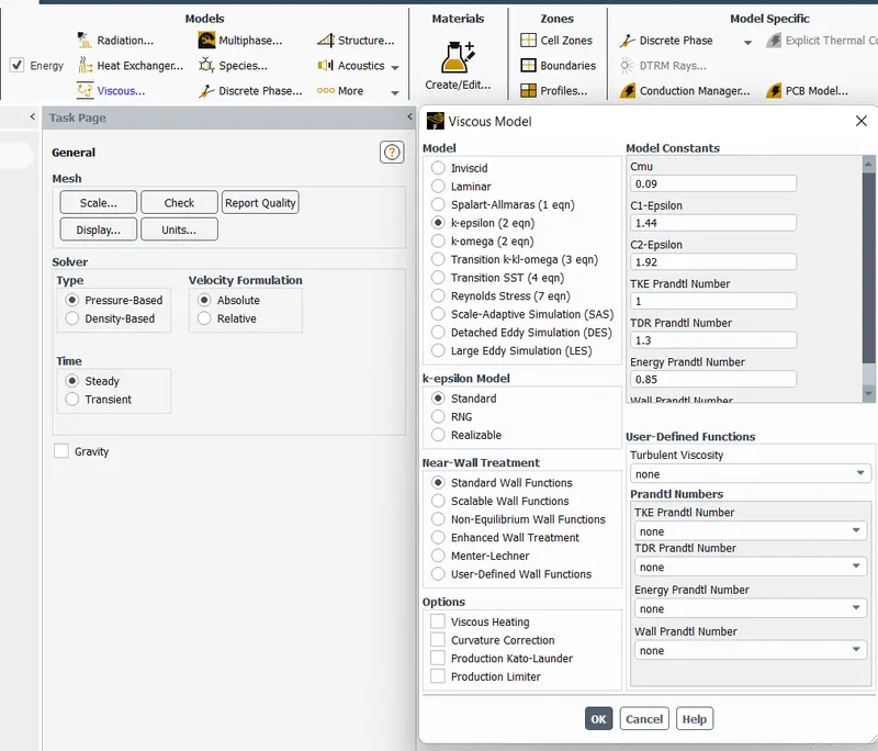
Then different materials are created using create/edit materials. After creating the materials, they are assigned to different components of the graphics card in the cell zones.
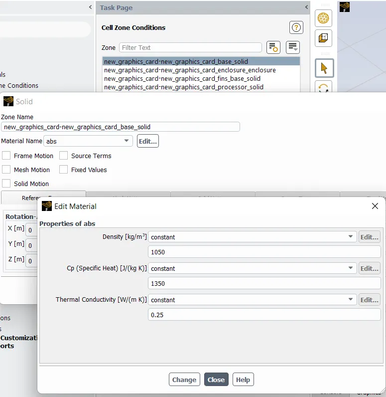
1. The base of the graphics card is assigned abs (Acrylonitrile butadiene styrene) with properties as shown below.
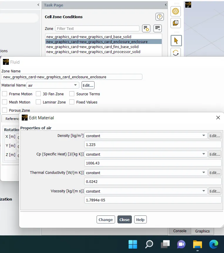
2. The enclosure is set as default fluid air.
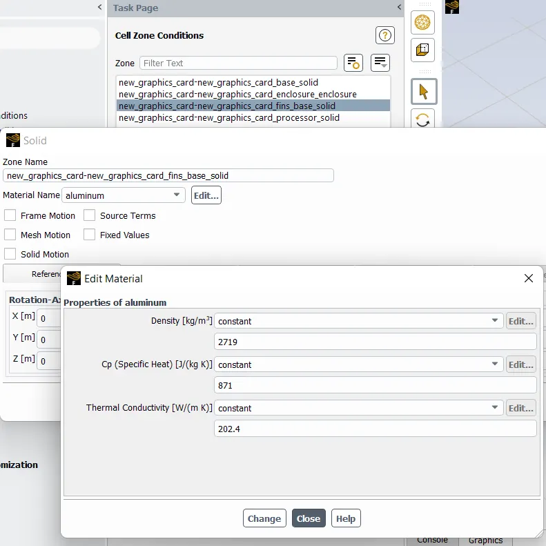
3. The fins of the graphics card are assigned as Aluminum with the properties as shown below.
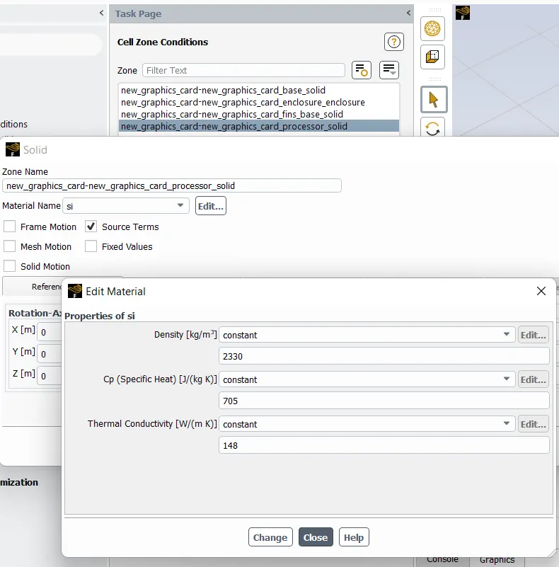
4. The processor of the graphics card is assigned as Silicon with the properties as shown below.
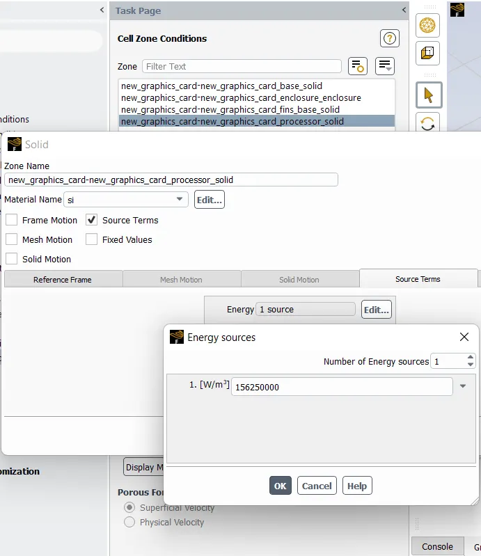
The heat generation takes place in the processor. So, the source terms option is checked and the value of thermal energy generated is given to be 156250000 W/m2 based on the below calculation.
Volumetric heat generated = Heat generated/volume of the processor
For a standard CPU, the heat generated by the processor is around 10 watts.
Volume of the processor = 8x8x1 = 64 x 10^-9 m3
Volumetric heat generated = 10 / 64x10^-9 =156250000 W/m2
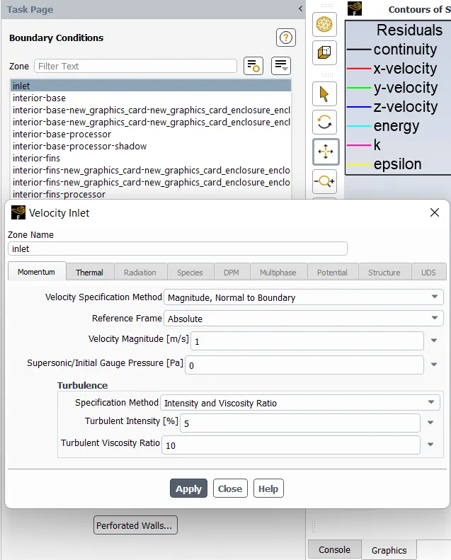
After setting up the cell zones we set up the boundary conditions i.e, velocity inlet as 1m/s, 3m/s, 5m/s, and pressure outlet.
Then hybrid initialization is done. Hybrid Initialization is a collection of recipes and boundary interpolation methods. It solves the Laplace equation to produce a velocity field that conforms to complex domain geometries, and a pressure field that smoothly connects high and low-pressure values in the computational domain. So, Hybrid initialization basically works on potential flow theory.
step-4 Solving and Results :
case-1: Baseline mesh
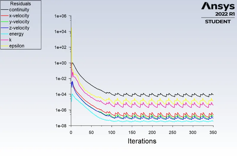
residuals
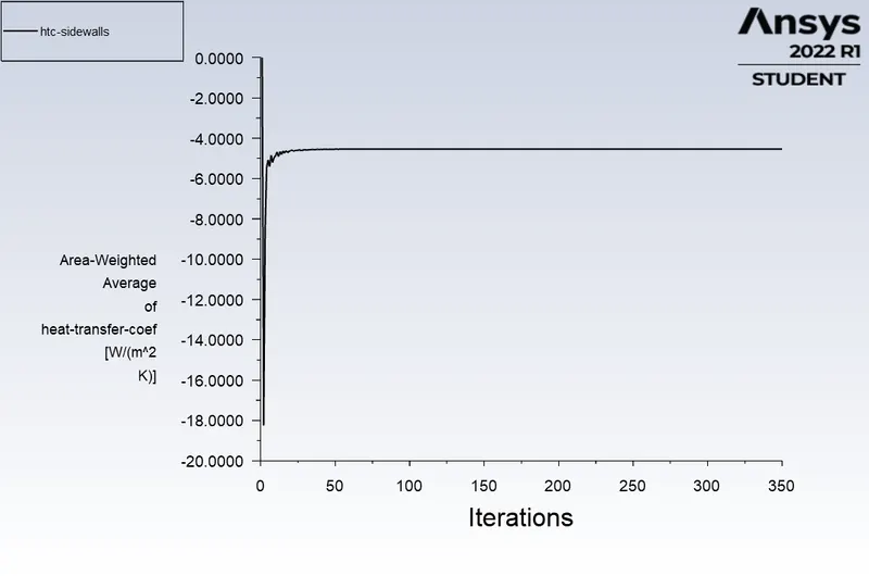
surface Heat transfer coefficient at sidewalls(processor)
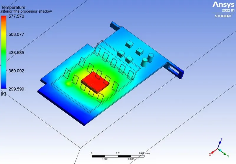
Temperature contour without fins
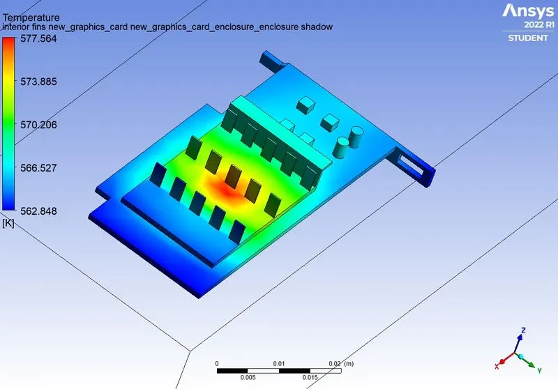
Temperature contour with fins
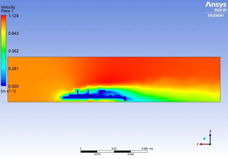
velocity contour across the length of the domain
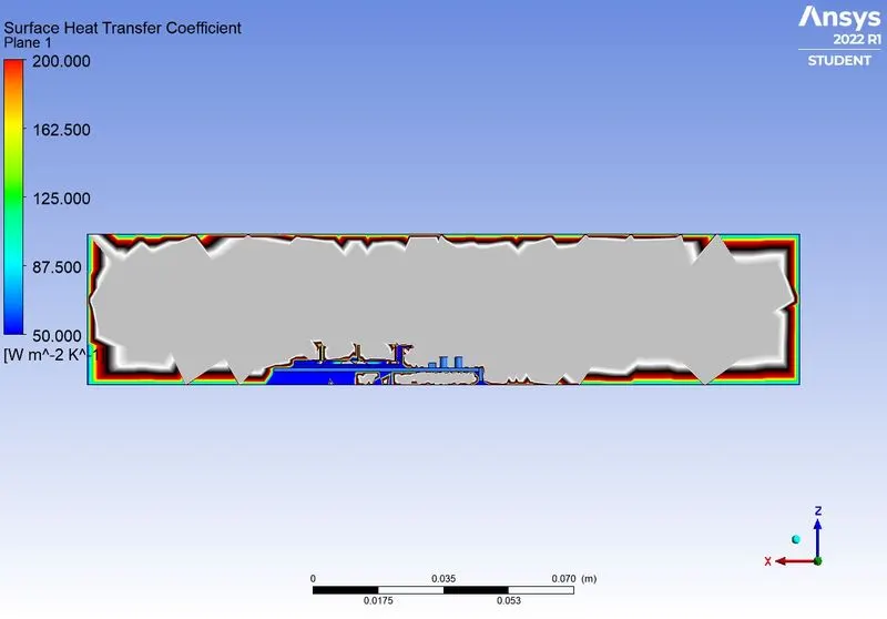
surface HTC across the length of the domain
case-3 : inlet velocity - 1m/s
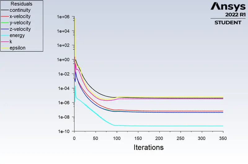
residuals
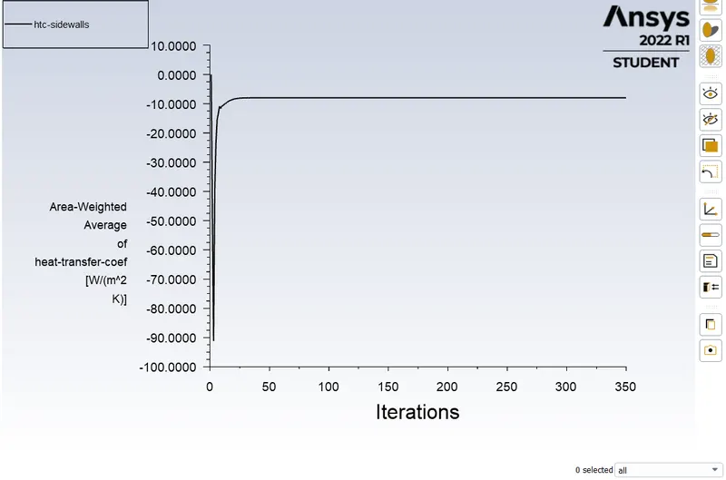
surface Heat transfer coefficient at sidewalls(processor)
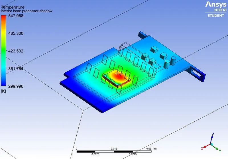
Temperature contour without fins
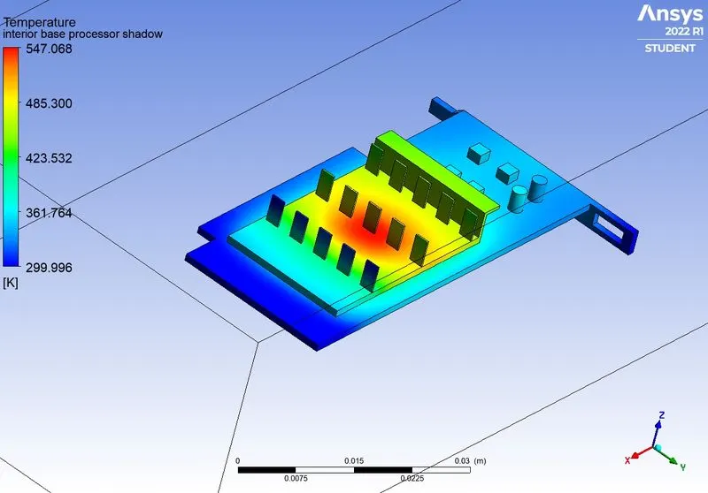
Temperature contour with fins
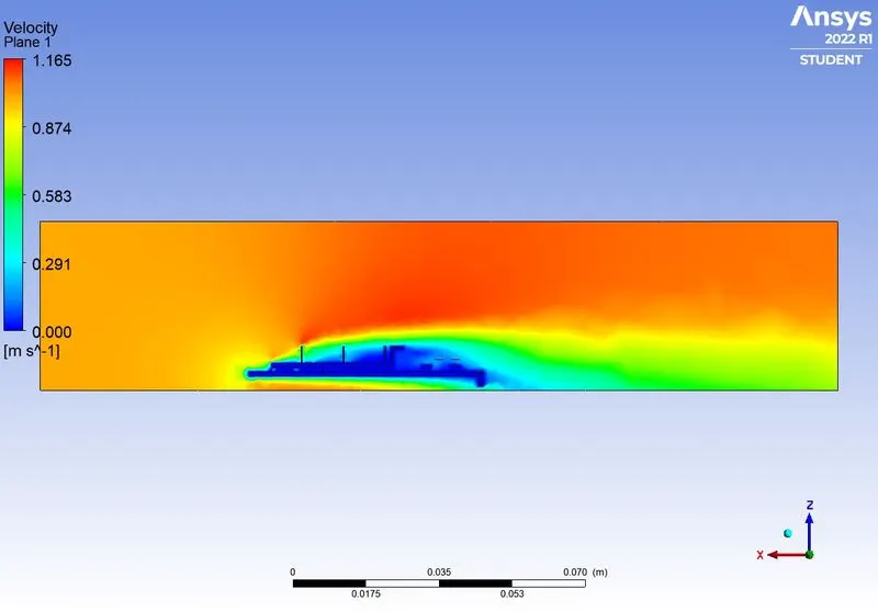
velocity contour across the length of the domain
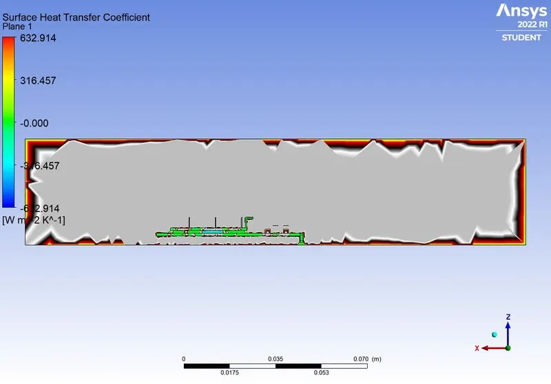
surface HTC across the length of the domain
case-3 inlet velocity - 3m/s
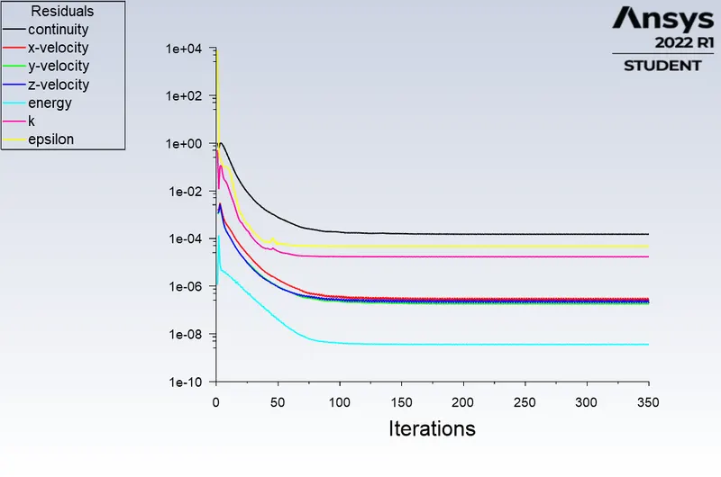
residuals
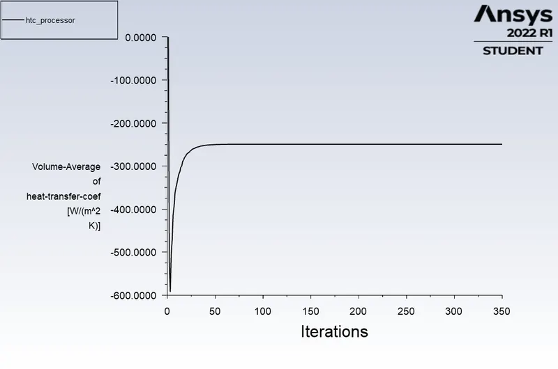
Heat transfer coefficient of the processor
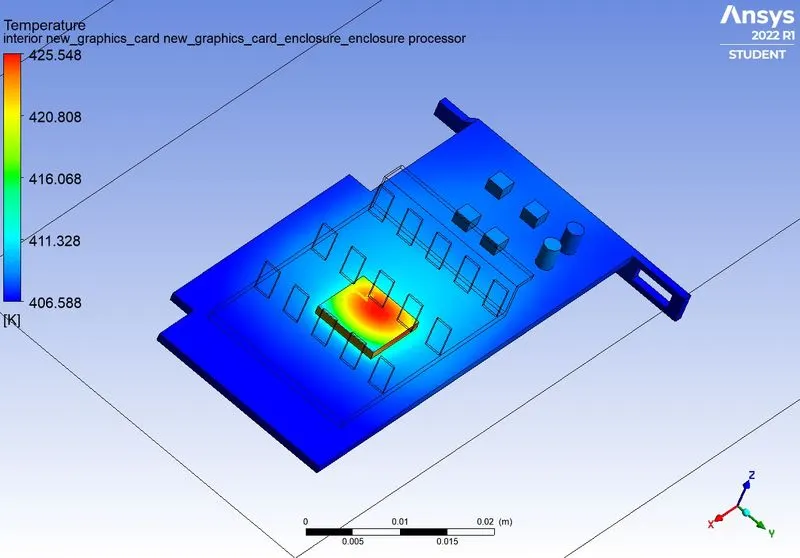
Temperature contour without fins
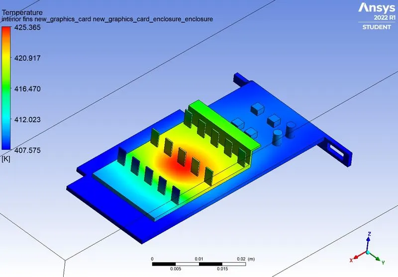
Temperature contour with fins
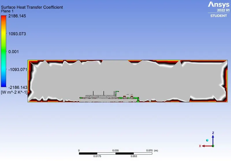
surface HTC across the length of the domain
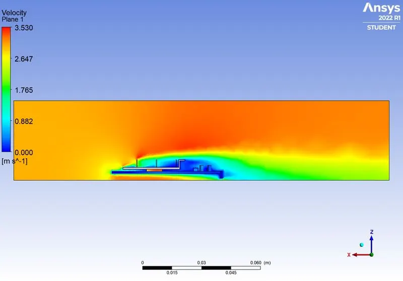
velocity across the length of the domain
case-4 : inlet velocity - 5m/s
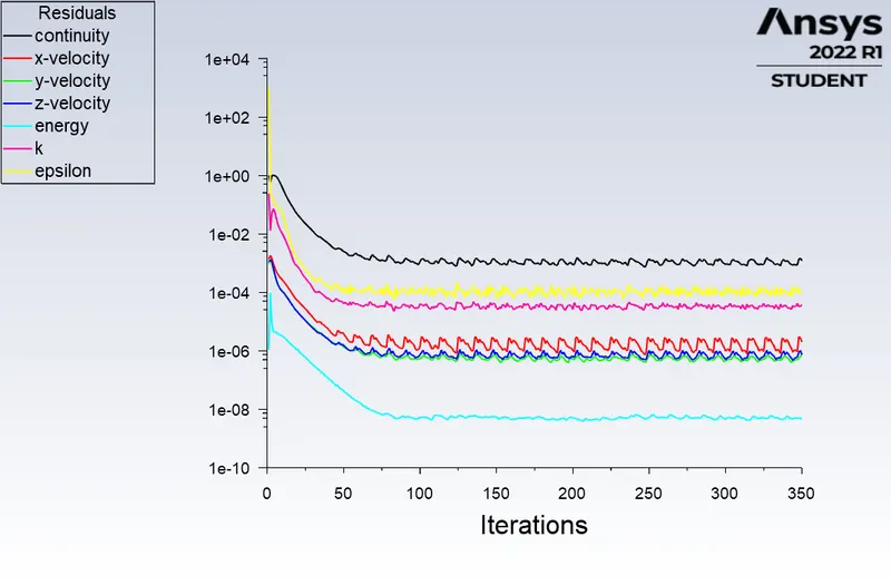
residuals
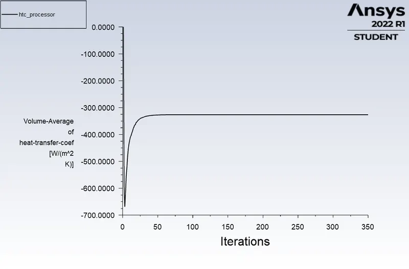
Heat transfer coefficient of the processor
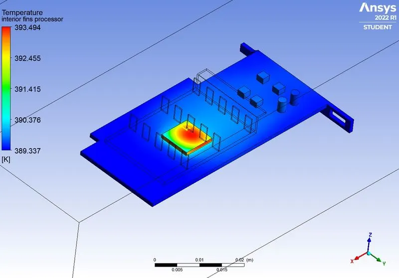
Temperature contour without fins
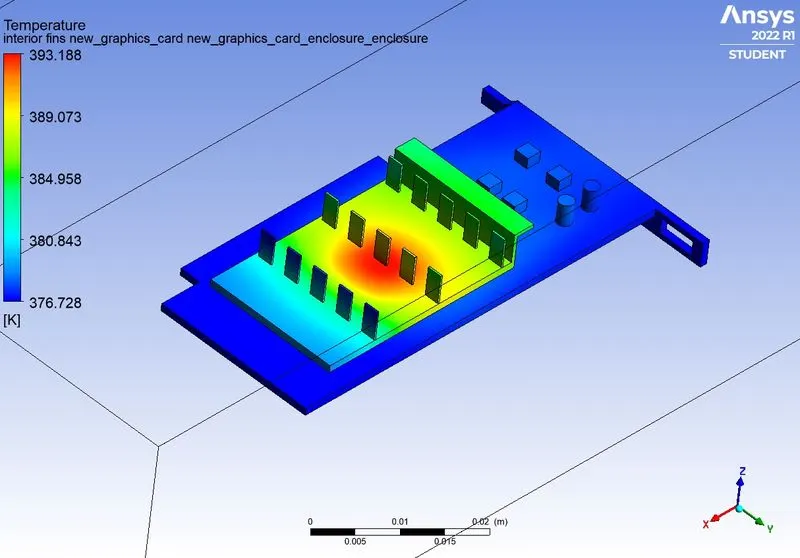
Temperature contour with fins
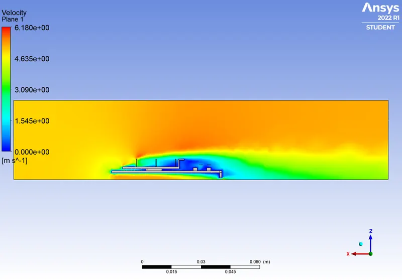
velocity across the length of the domain
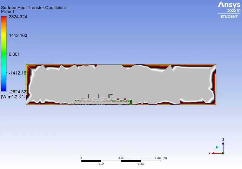
surface HTC across the length of the domain
Observation and Conclusion :
| velocity | surfaceHtc sidewalls (W/m2 K) | Temp processor(K) | |
| case1 | 1 | -4.5395551 | 577.4561 |
| case 2 | 1 | -7.978411 | 544.9435 |
| case 3 | 3 | -13.2985 | 424.7921 |
| case4 | 5 | -19.23763 | 392.6653 |
1. The potential hotspots can be identified from the temperature contours i.e, the area particularly near the processor.
2. In this case, for the solution to reach convergence, not only the residuals but also the HTC graph is also analyzed.
2. When the velocity increases, the heat transfer coefficient also increases. So, the temperature of the processor decreases.