Week 4 - CHT Analysis on Exhaust port
Aim :
1. To perform conjugate heat transfer analysis on the Exhaust port.
2. To create inflation layers maintaining the y+ value according to the turbulence model chosen.
3. To perform a validation study.
Introduction:
The exhaust manifold, which collects engine exhaust gas from multiple cylinders and delivers it to the exhaust pipe, forms one of the vehicle's main components. A poorly functioning exhaust system means lower fuel efficiency, and decreased power, and could even lead to costly damage down the line. If the temperature fields are not monitored properly it could lead to weak areas, like joints, cracking, and leaking poisonous fumes into the passenger cabin resulting in serious health and safety issues.
Conjugate heat transfer corresponds with the combination of heat transfer in solids and heat transfer in fluids. In solids, conduction often dominates whereas, in fluids, convection usually dominates. Conjugate heat transfer is observed in many situations. For example, heat sinks are optimized to combine heat transfer by conduction in the heat sink with the convection in the surrounding fluid.
Typical applications of this analysis type exist as, but are not limited to, the simulation of heat exchangers, cooling of electronic equipment, and general-purpose cooling and heating systems.
Natural convection around a heat exchanger. Cold water enters in and gets heated due to hot air flowing opposite to it
The basic transport equation which is solved to calculate the internal/thermal energy is,
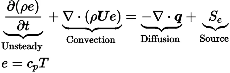
The transport equation in terms of 'T' and substituting heat flux (q)=-thermal conductivity(k)*temperature gradient(dt) is given by,
 ---------------------> (1)
This works fine for the incompressible flows(pressure-based solver). But this is not sufficient for compressible flows where the flow speed is high.
So, the internal energy is converted into mechanical/kinetic energy from the Navier-Stokes equation.
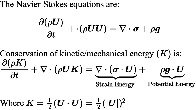
The transport equation for the total energy which accounts for both the internal energy and kinetic/mechanical energy is given by,
Total energy(E) = internal energy(e) + kinetic/mechanical energy(k)
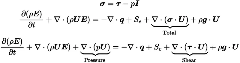
The total shear stress tensor(σ) is decomposed into shear(tau) and normal pressure components.
Heat Transfer in a Solid
In most cases, if only due to conduction, heat transfer in solids is described by Fourier’s law defining the conductive heat flux, q, proportional to the temperature gradient:  .
.
For a time-dependent problem, the temperature field in an immobile solid verifies the following form of the heat equation:
 represents the (1) when u=0
 Heat Transfer in a Fluid
Due to the fluid motion, three contributions to the heat equation are included:
- The transport of fluid implies energy transport too, which appears in the heat equation as the convective contribution. Depending on the fluid's thermal properties and the flow regime, either the convective or the conductive heat transfer can dominate.
- The viscous effects of the fluid flow produce fluid heating. This term is often neglected, nevertheless, its contribution is noticeable to fast flow in viscous fluids.
- As soon as a fluid density is temperature-dependent, a pressure work term contributes to the heat equation. This accounts for the well-known effect that, for example, compressing air produces heat.
Accounting for these contributions, in addition to conduction, results in the following transient heat equation for the temperature field in a fluid:

In any CFD analysis, the workflow that is followed is
Setting up the geometry ----> Meshing ----> setting up the solver ---->solving ---->post-processing results
step-1 Setting up the geometry :
First, the pre-designed exhaust port geometry is imported into Spaceclaim. The geometry is a solid model through which the exhaust gases flow.
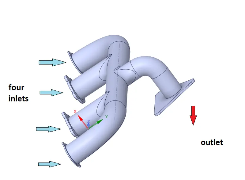
The extra/duplicate edges are removed using the extra edges feature. The extra edges interfere while selecting the faces which capture the fluid volume. Then volume extract feature is used to extract the flow volume .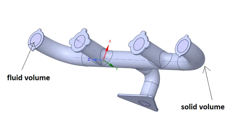
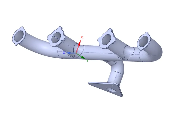
solid volume
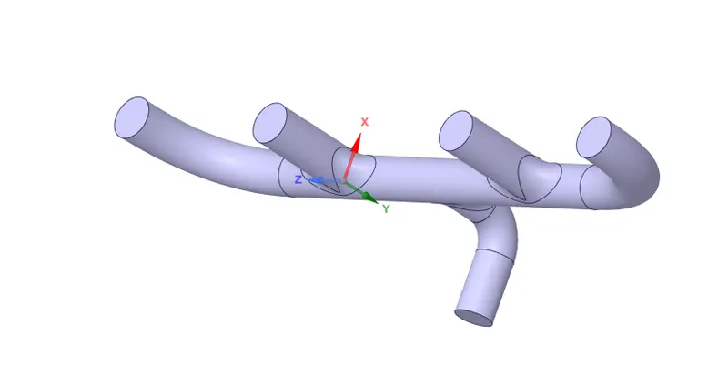
fluid volume
After extracting the fluid volume, the share topology is turned on, which enables information transfer between both bodies. Then the shareprep tool is used to create the common/co-incident interfaces between both the bodies.
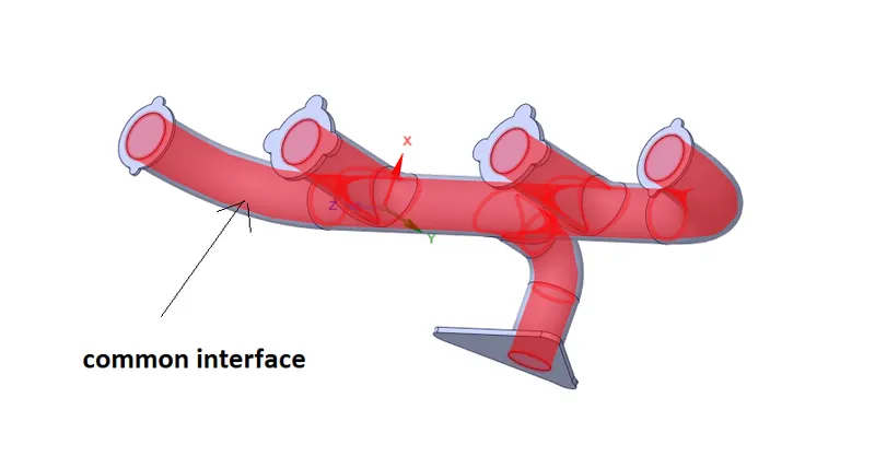
step-2 Creating the mesh:
case-1 Baseline mesh :
Meshing is the process of generating a grid i.e, dividing complex geometries into elements that can be used to discretize a domain. First, a baseline mesh is generated(i.e, without changing any parameters) to check the solver settings. If the flow physics works fine, then the mesh refinement is done.
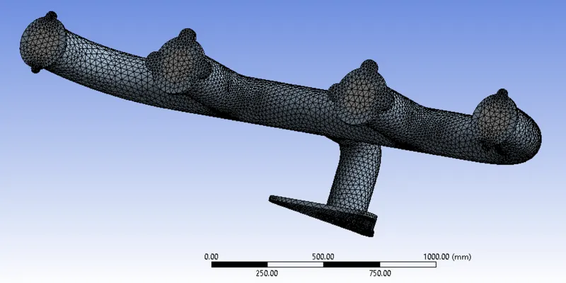
First, a baseline mesh(tetra mesh) is generated which consists of 138265 elements and 27541 nodes.
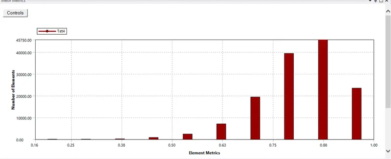
Then the quality of the mesh is checked using the mesh metric in mesh settings, which shows that most of the elements fall above 0.8(1 being the perfect tet-4 element) and the least elements fall below 0.16, which is perfectly fine for a base mesh.
When we closely observe the mesh at the interfaces, the mesh perfectly aligns(conformal mesh). The information transfer takes place in a smooth manner with this type of mesh.
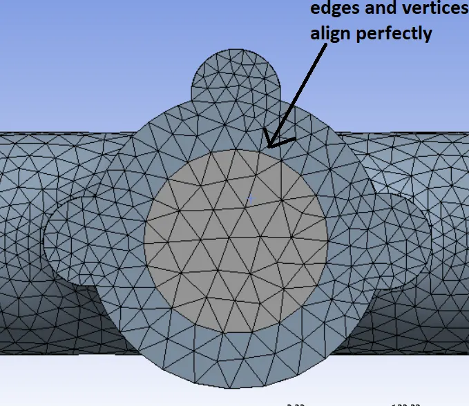
conformal mesh
Then the boundaries are named by selecting a particular face and naming it accordingly.
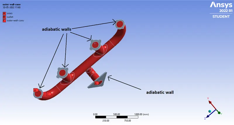
The remaining walls are not given any names. However, fluent automatically assigns them as walls(which do not transfer heat, adiabatic walls).
case -2 Mesh Refinement :
First, the mesh is generated. On top of that other meshing strategies are added. In this case, the element size of the solid volume is changed to 10mm by the Bodysizing method. Similarly, again using the Bodysizing method the element size of the fluid volume is refined to 15mm.
The near-wall modeling significantly impacts the solution, as the walls are the main source where the mean vorticity and turbulence vary. After all, it is in the near-wall region that the solution variables have large gradients, and the momentum and other scalar transports occur most vigorously. Therefore, accurate representation of the flow in the near-wall region becomes of utmost importance.
So, inflation layers or body-fitted mesh are created along the fluid volume.
Mesh settings --> Inflation --> choose the outer region of the fluid volume(named selection) --> total thickness --> number of layers:7 --> maximum thickness : 17.4mm --> generate mesh
The total thickness of the inflation layers is calculated using the below formulae :

As we are working with the k-epsilon turbulence model( based upon the inbuilt wall functions), to capture the near-wall phenomena the desired y+ ranges from 30 to 300.
So, desired y+ value was chosen as 100 and the total thickness of the layers came out to be 17.4mm.
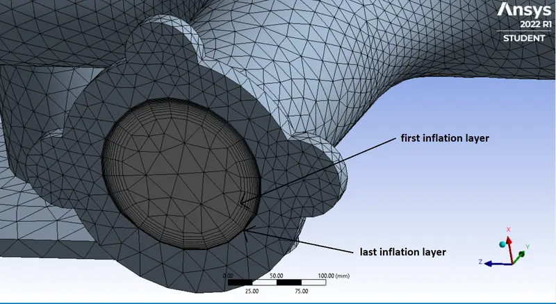
inflation layers
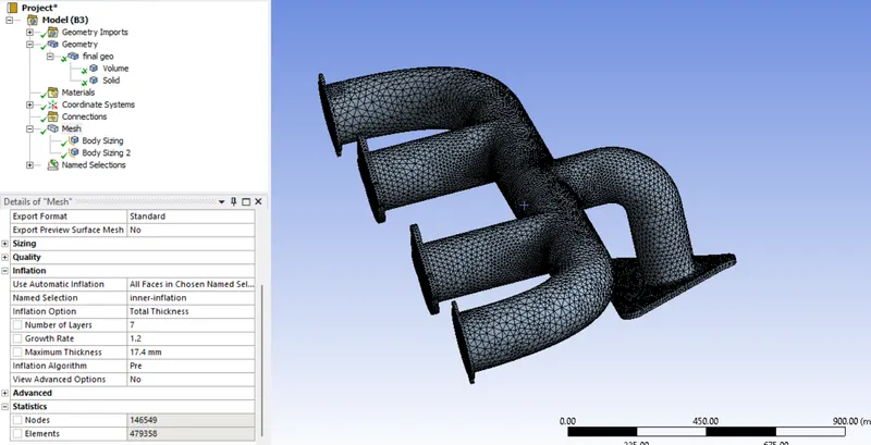
3D view of the refined mesh geometry
number of elements - 0.47 million cells
number of nodes - 0.14 million nodes
step-3 Setting up the solver in Ansys FLuent:
In this step, we define various parameters like initial and boundary conditions, materials used, time steps(for transient), turbulence model, etc which captures the physics to be simulated.
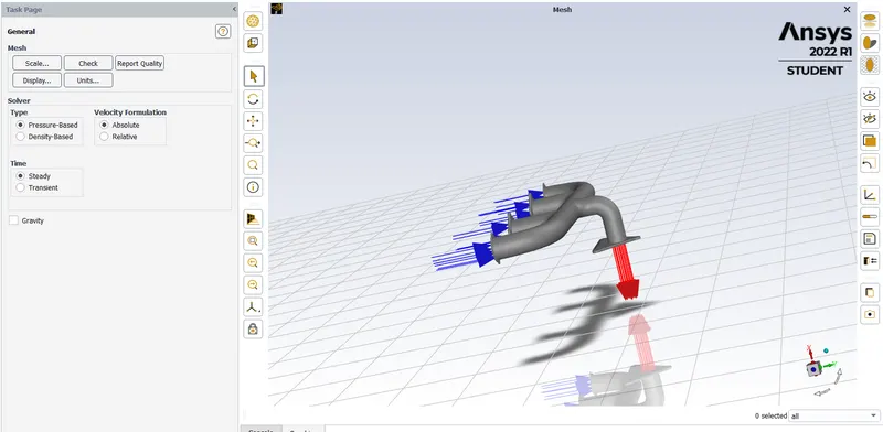
First, we set up the physics by choosing the pressure-based solver which was particularly designed for low-speed incompressible flows(low Mach number), while the density-based solver was mainly designed for high-speed compressible flows(high Mach number).
Then, the steady-state solver is checked, as we are interested in seeing the final results after the flow variables become steady. Along with the standard governing PDEs, we will also be solving the Energy equation.
The turbulence model is selected as the k-epsilon model i.e, the standard k-epsilon model with standard wall function, which solves for turbulence kinetic energy 'k' and its dissipation rate 'epsilon'.
In the case of materials, for solid, we choose 'aluminum' material whereas 'air' is chosen as the fluid material.
Then the boundary conditions are defined.
Inlet : velocity - 5m/s , Temperature - 700K
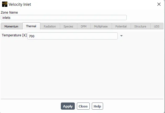
Outlet - pressure outlet
outer wall convection: heat transfer coefficient - 20W/m^2.K
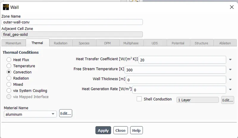
Then as the final step, hybrid initialization is done. Hybrid Initialization is a collection of recipes and boundary interpolation methods. It solves the Laplace equation to produce a velocity field that conforms to complex domain geometries, and a pressure field that smoothly connects high and low-pressure values in the computational domain. So, Hybrid initialization basically works on potential flow theory.
step-4 Solving and Results :
case-1 :
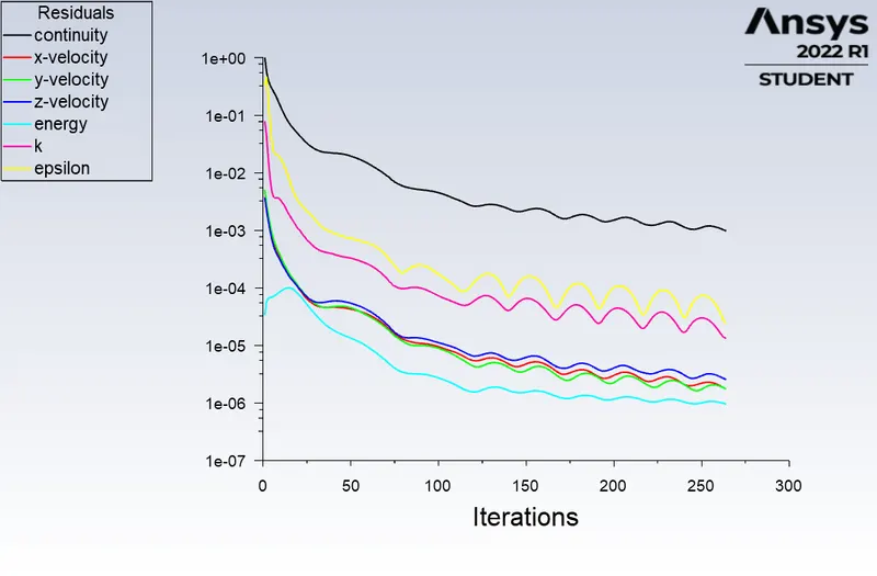
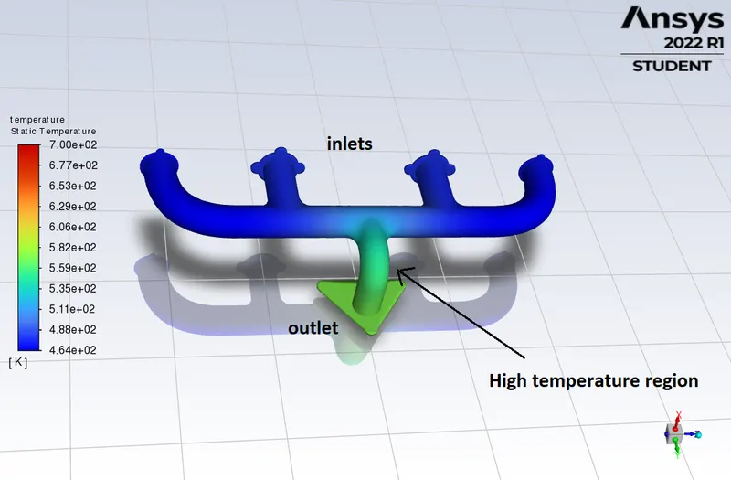
Temperature contour
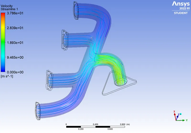
velocity streamline
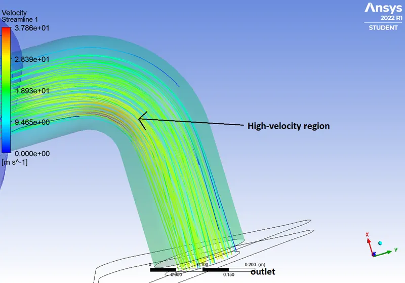
high-velocity region near the outlet
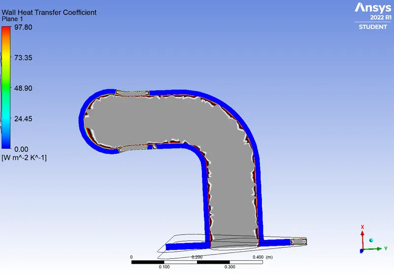
Wall heat transfer coefficient
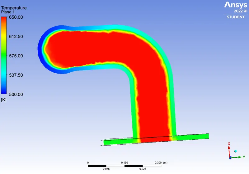
temperature contour near the outlet
case-2:
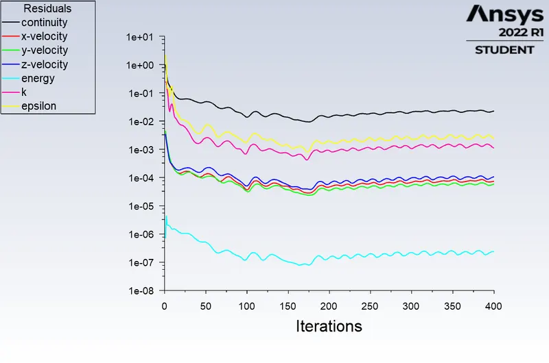
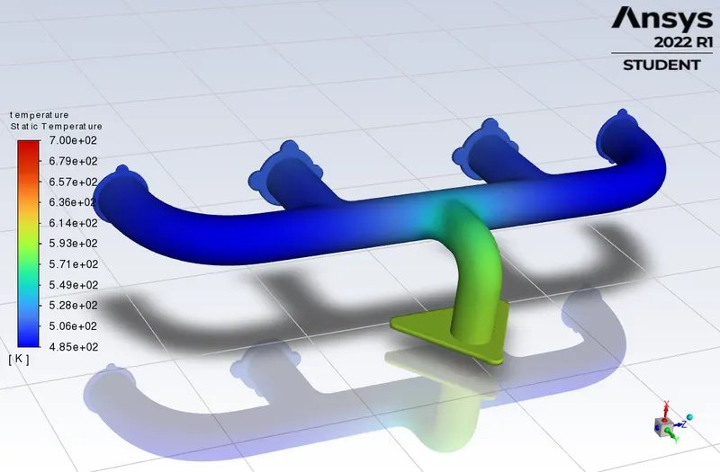
temperature contour
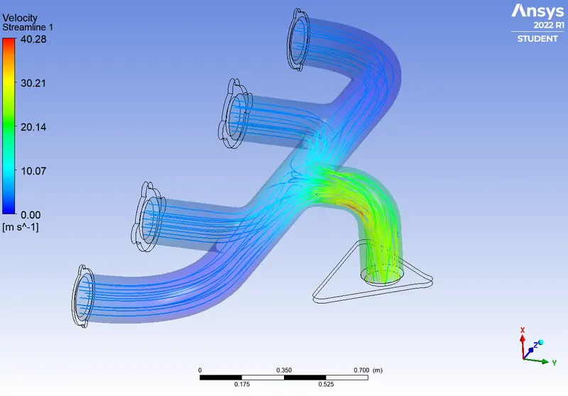
velocity streamlines
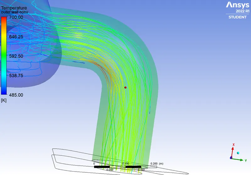
high-velocity region near the outlet
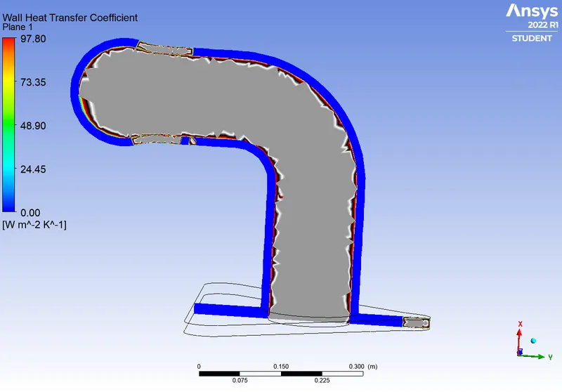
Wall heat transfer coefficient near the outlet
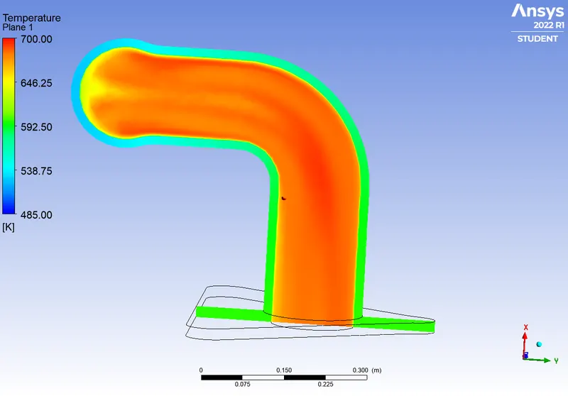
temperature contour near the outlet
Observation and Conclusion :
1. From the velocity streamlines plot we can observe that the velocity near the outlet is the highest which indicates that, to conserve the mass flow rate, the velocity increases at the outlet.
2. The HTC at the high velocity region is the highest which indicates that, to conserve the temperature flux, the heat transfer rate near the outlet increases.
3. The HTC plot, temperature contours from both the cases show almost the same result.But with adding inflation layers, we capture the near wall phenomena accurately.
Validation Study :
The most common and most popular numerical modeling technique is computational fluid dynamics, which became quite popular in the 1970s, 1980s, and 1990s with the increasing power of computers. CFD modeling is based on the principles of fluid mechanics, utilizing numerical methods and algorithms to solve problems that involve fluid flows. Models attempt to simulate the interaction of liquids and gases.CFD models are based on the principles of the Navier–Stokes equations. Simulations are then conducted by solving the equations iteratively as steady-state or transient.
As numerical models, approximate real-world problems into a bunch of assumptions and solves them iteratively. A question strikes how am I to rely on this numerical model? The validity of these models is usually established by benchmark testing. This is done to quantitatively measure the agreement between the predictions provided by the model and the real world represented by observations in experiments. This approach assumes that all variables in the real world relevant for the specific study are adequately measured in the experiments and the predictions made by the model.
In this case of heat transfer analysis, to validate the numerical result, the heat transfer coefficient is compared with the analytical result. the heat transfer coefficient is used for calculating heat transfer between a fluid and a solid.
h = ∆Q/(A * ∆T * ∆t)
where h is the heat transfer coefficient, ∆Q is the heat input into the system or the heat lost, A is the surface area where the heat is transferred, ∆T is the temperature difference between the sold surface and the surrounding fluid area, and ∆t changes in time comprising the time period in which the heat transfer has occurred.
Most solid substances have a known thermal conductivity which can be used as a basis for calculating the heat transfer coefficient. A very common engineering problem is the heat transfer between a fluid and a solid surface. The most common way of doing this is by dividing the thermal conductivity of the convection fluid by a length scale. It is also common to calculate the coefficient with the Nusselt number (one of several dimensionless groups used in fluid dynamics).
h = Nu * k / l
Nu is the Nusslet number which is a dimensionless number used in convective heat transfer analysis. The Nusselt number is the ratio of heat transfer by convection to the heat transfer by conduction within a fluid (When the fluid is considered stationary).
`Nu = Q_(conve ction)/Q_(conduction)`
`Q_(conve ction)= h*A*DeltaT`
`Q_(conduction)= k*A*(DeltaT)/L`
`Nu= (hL)/k`
For the forced convection, the equation of the Nusselt number is written in the form of Reynolds number and Prandtl number as,
`Nu=c(Re)^m (Pr)^n`
Where the values of C, m, and n are determined experimentally for different conditions.
Significance of Nusslet number:
1] The Nusselt number gives the relation between heat transfer by conduction and heat transfer by convection.
2] When Nu = 1, It means that the rate of heat transfer by conduction is equal to the rate of heat transfer by convection or we can say that fluid is stationary.
3] If the Nu > 1, Then the heat transfer by convection is greater than the heat transferred by conduction.
A very widely used empirical relation for heat transfer coefficient in a fully developed turbulent flow through a pipe was given by Dittus and Boelter. According to them,
`Nu=0.023*(Re)^(0.8)*(Pr)^(0.4)`
`Re = (v*L)/nu`
`Pr = nu/alpha=(mu C_p)/k`
The value of the Prandtl number tells us by what means the heat would diffuse faster, i.e., whether heat conduction is more dominant than convection for a fluid.
Calculation :
diameter of the pipe(L)=166*10^-3 m
density of air(rho)=1.225kg/m3
specific heat = 1006.43 J/kg K
thermal conductivity(k) = 0.0242 W/ m K
dynamic viscosity(nu) = 1.7894e-05 Pa-s
To calculate the HTC at the high-velocity region
u = 37 m/s
`Re = (v*L)/nu`
`Re =( 37* 166*10^-3)/(1.7894e-05) = 420473`
`Pr = nu/alpha=(mu C_p)/k = (0.0000182*1006)/0.0242=0.7156`
`Nu=0.023*(Re)^(0.8)*(Pr)^(0.4) = 0.023*(420473^0.8)*(0.7156^0.4)=634.7262`
`h = (k*Nu)/L=(0.0242*634.726)/(166*10^-3)= 92.532 W/(m^2 K)`
Numerical HTC at the high-velocity region = 97 W/m^2 K
Error = 5.38 %