Week 9 - Parametric study on Gate valve.
Aim:
1. To perform fluid flow simulation on the gate valve.
2. To parameterize the lift distance from 10mm to 80mm and analyze the mass flow rate at the outlet.
Introduction :
A gate valve is a control valve that regulates the fluid flow accordingly. The main advantage of a gate valve is the straight-through unobstructed passageway, which induces minimal pressure loss over the valve. A gate valve is made up of 5 main components - Hand wheel, spindle, bonnet, gate disc, and bottom.
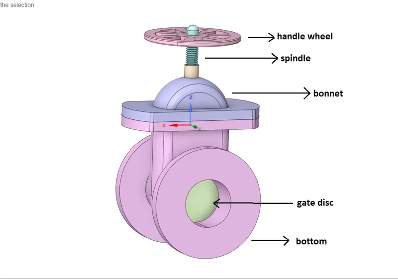
To open the valve, the handwheel is turned, which moves the gate disc vertically. When the gate disc is lifted, it opens the inlet to the outlet allowing the fluid flow. When the gate disc is lowered, it closes and blocks the fluid flow.
In any CFD analysis, the workflow that is followed is
Setting up the geometry ----> Meshing ----> setting up the solver ---->solving ---->post-processing results
step-1 Setting up the geometry :
First, the pre-designed gate valve geometry is imported to the SpaceClaim module, to extract the fluid volume.
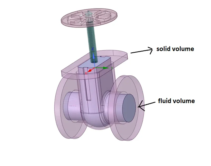
After fluid volume extraction
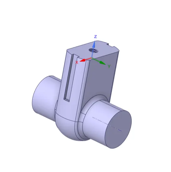
fluid volume
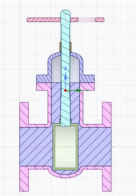
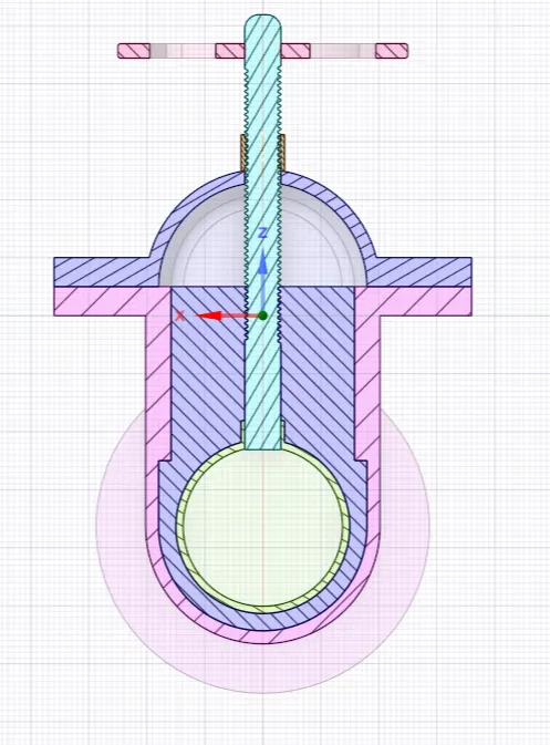
front view at the closed position side view at the closed position
For the first case, the gate disc has to be lifted 10mm in the z-direction, which is done using the move feature.
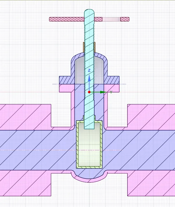
front view (first case, lift =10mm)
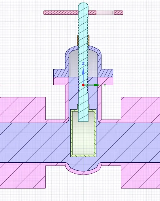
second case, lift =20mm
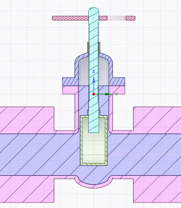
third case, lift =30mm
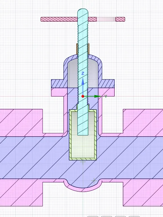
fourth case, lift =50mm
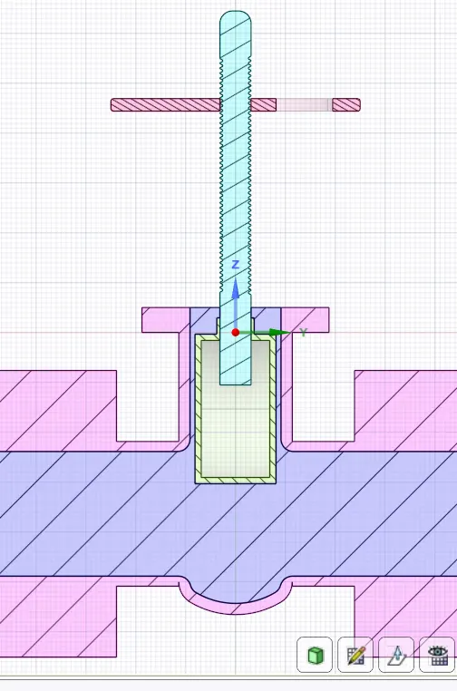
fifth case, lift =80mm
The inlet and outlet are extended to 800mm, using the pull feature.
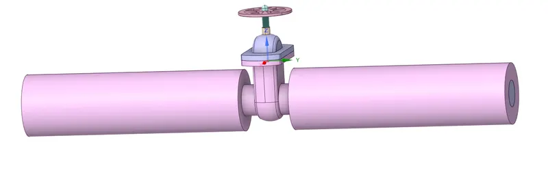
Then the fluid volume is updated as per the geometry changes.
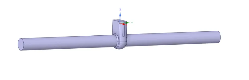
The solid volume is suppressed for physics, as we are only interested in simulating the flow.
step-2 Creating the mesh:
Meshing is the process of generating a grid i.e, dividing complex geometries into elements that can be used to discretize a domain. An automated mesh with an element size of 10mm is generated, which consists of 193398 elements, and 38787 nodes.
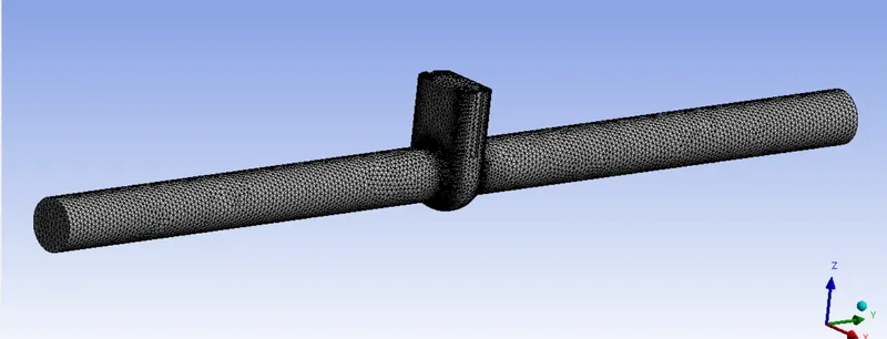
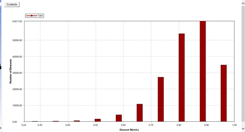
Then the quality of the mesh is checked using the mesh metric in mesh settings, which shows that most of the elements fall above 0.8(1 being the perfect tet-4 element) and the least elements fall below 0.50, which is perfectly fine.
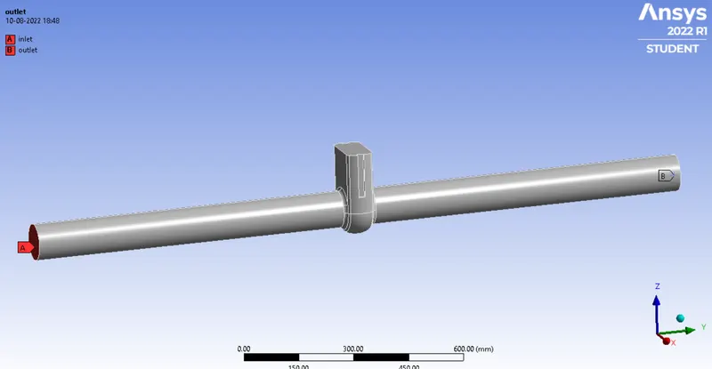
Then appropriate faces are selected and named accordingly.
step-3 Setting up the solver in Ansys Fluent:
In this step, we define parameters like initial and boundary conditions, materials used, time steps(for transient), turbulence model, etc., which captures the physics to be simulated.
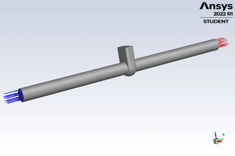
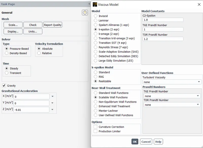
First, we set up the physics by choosing the pressure-based solver which was particularly designed for low-speed incompressible flows(low Mach number), while the density-based solver was mainly designed for high-speed compressible flows(high Mach number).
Then, the steady-state solver is checked, as we are interested in seeing the final results after the flow variables become steady. The gravity field is enabled, along the negative z-direction.
For the turbulence model, the k-epsilon realizable model with scalable wall functions is selected.
Water-liquid is copied from the fluent database and assigned as the fluid.
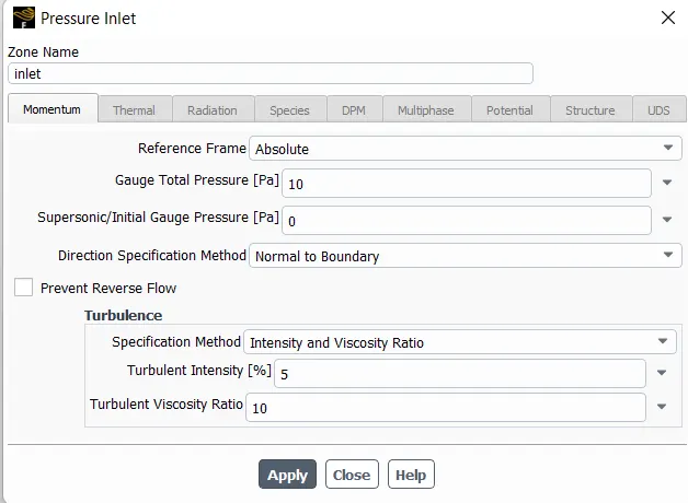
The inlet boundary condition is changed from velocity inlet type to pressure inlet, with a value of 10 bar gauge pressure.
The outlet boundary condition is left as the default i.e, pressure outlet type with zero gauge pressure.
The initial values are computed from the inlet using standard initialization.
Before running the solver, reports for calculating the mass flow rate at the outlet, pressure drop across the gate valve, and velocity contours across the geometry are created. Then the solver is run for 300-400 iterations.
Results:
A. Residuals:
case-1: lift distance=10mm
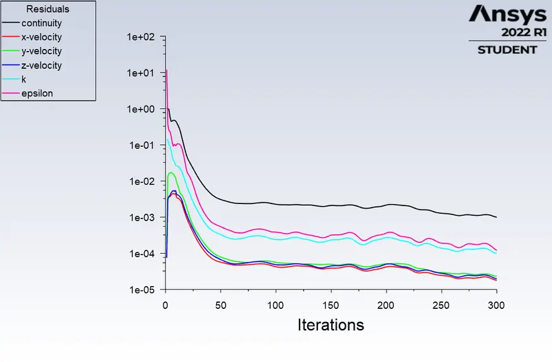
case-2: lift distance=20mm
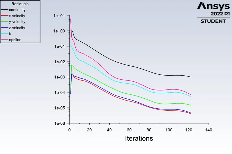
case-3: lift distance=30mm
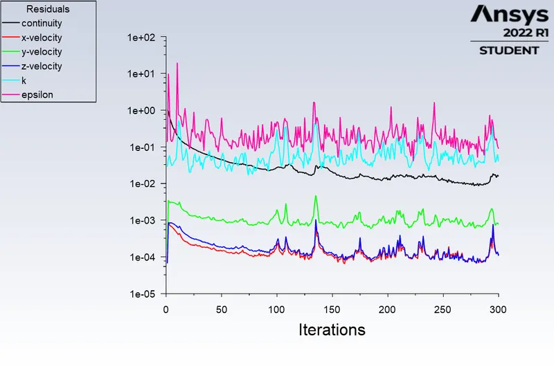
case-4: lift distance=50mm
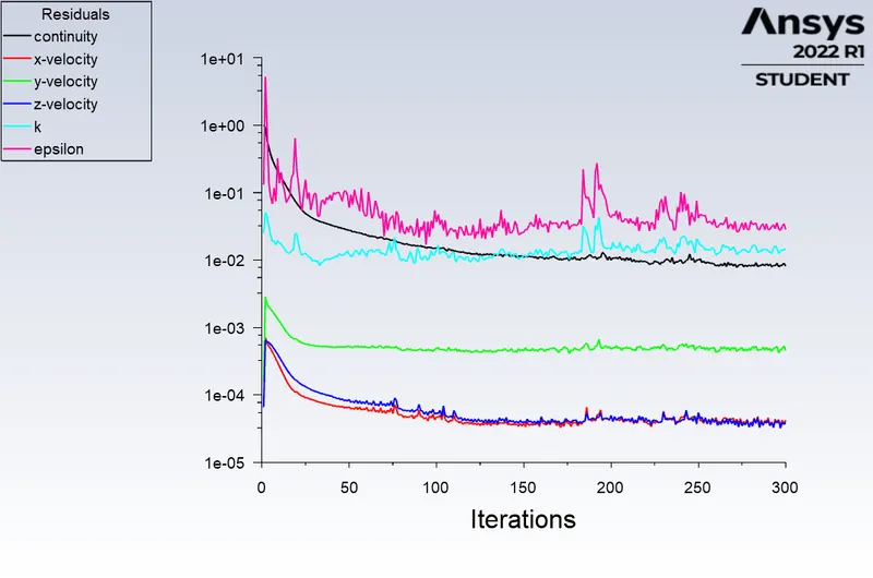
case-5: lift distance=80mm
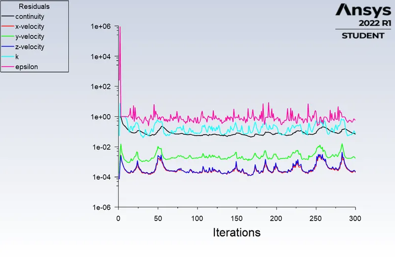
B. Mass flow rate
case-1: lift distance=10mm
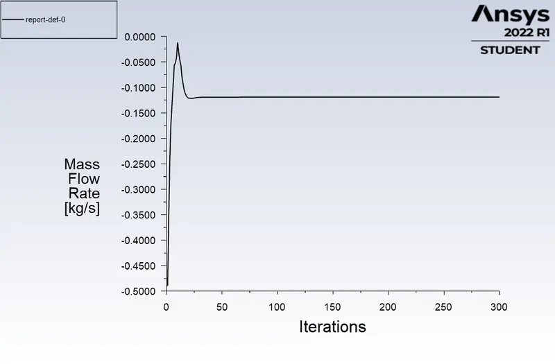
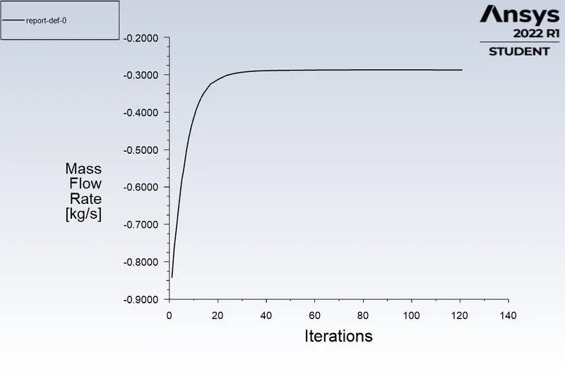
case-2: lift distance=20mm
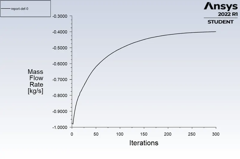
case-3: lift distance=30mm
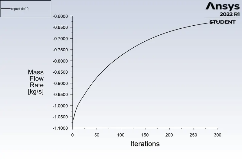
case-4: lift distance=50mm
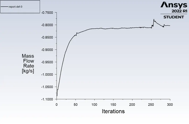
case-5: lift distance=80mm
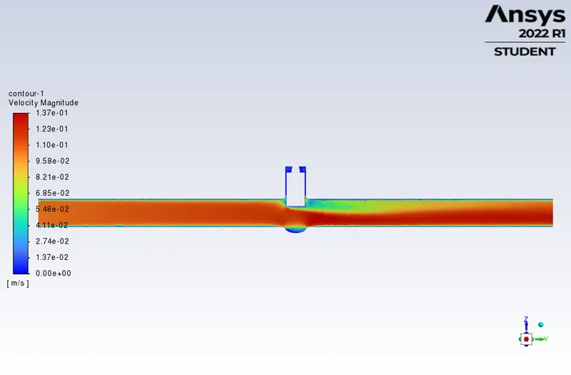
C. Velocity contours
case-1: lift distance=10mm
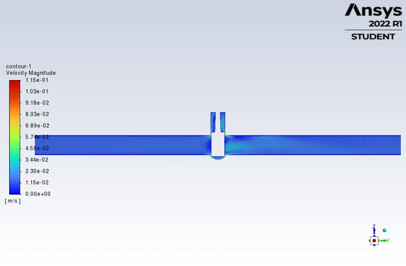
case-2: lift distance=20mm
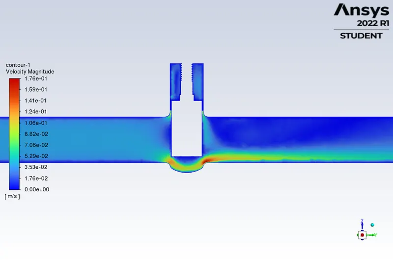
case-3: lift distance=30mm
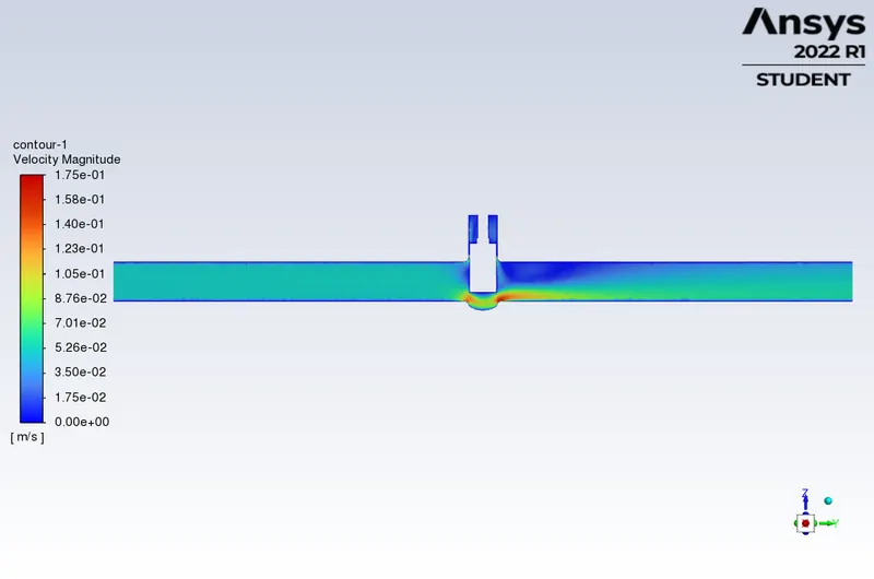
case-4: lift distance=50mm
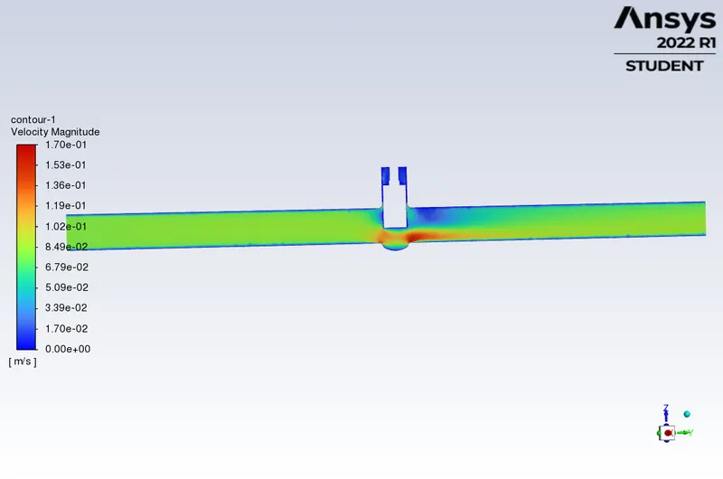
case-5: lift distance=80mm
Flow factor
`k_v=Qsqrt((SG)/(DeltaP))`
where Q - flow rate ( m^3/hr)
flow rate = mass flow rate (kg/hr) / density(kg/m3)
SG - specific gravity ( for water=1)
`DeltaP`- pressure drop across the gate valve (bar)
The valve flow factor is an essential measurement that helps you calculate how much fluid can pass through a valve.
Observations and Conclusion:
| lift | mass flow rate | flow rate(m3/hr) | inlet pressure | outlet pressure | pressure drop | flow factor | |
| case1 | 10mm | -0.18077 | -0.652722897 | 9.731529 | 0 | 9.731529 | 0.033537 |
| case2 | 20mm | -0.287 | -1.036321926 | 9.323457 | 0 | 9.323457 | 0.055576 |
| case3 | 30mm | -0.39902 | -1.440803338 | 8.686716 | 0 | 8.686716 | 0.082931 |
| case4 | 50mm | -0.62539 | -2.258184638 | 6.763263 | 0 | 6.763263 | 0.166945 |
| case5 | 80mm | -0.8036 | -2.901655787 | 4.676994 | 0 | 4.676994 | 0.310205 |
1. When the lift was increased, the mass flow rate also increased.
2. When the lift was increased, the pressure drop across the gate valve decreased.
3. On accounting for the two factors, the flow factor had been calculated and observed that when the lift was increased, the flow factor also increased.