Calculation of State Variables & Efficiency of Gas Power Cycle (Otto Cycle)

Contents

1. Introduction to Gas Power Cycle
2. Primary assumptions for Otto Cycle
3. Comparing P-V & T-S characteristic curves with SI Engine cycle
4. Efficiency calculation for Otto Cycle
5. MATLAB coding for calculation of state variables & PV plot generation for Otto Cycle
6. Explanation of Code & Syntax usage
7. Errors committed while coding

1. Introduction to Gas Power cycle:

Power cycles are classified based on the usage of working fluids as the medium to generate Power, transfer & transform heat in the closed system of a cyclic process loop. Based on the usage of working fluids the power cycles are classified into

1. Vapour Power Cycle – The working fluid in this cycle undergoes a phase change in the closed cyclic loop process. (Water)

2. Gas Power Cycle – The working fluid does not undergo any phase change in the closed cyclic loop process & the working fluid/medium is considered to be Air assuming it to be behaving like Ideal Gas. Hence the name Air Standard Cycle

Ideal Cycle (Air Standard Cycle) Block diagram for Work-done

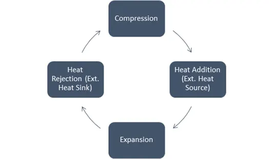
Real-life Cycle (IC Engine/Gas Turbine) Block diagram for Work-done

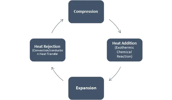
Primary assumptions in Otto Cycle

Major assumptions in Otto cycle are as follows:

1. Air itself alone is considered to be the working fluid in the cyclic process. Even though during combustion process, the products of combustion are not accounted as the working fluids
2. Air is considered to be following the governing equations of Ideal Gas Laws
3. Presence of Thermal Equilibrium & internal reversibility of system
4. Heat addition is done by a separate heat source from outside the system
5. Heat is rejected to a separate heat sink outside the system

3. P-V & T-S Characteristic curves for Otto Cycle in comparison with SI Engine cycle:

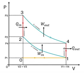
Process 0-1: (Constant Pressure Air Induction)

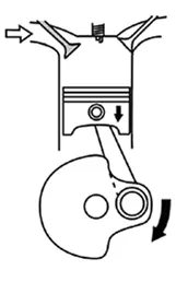
Due to descending motion of the piston in the downward direction, the air present in the combustion chamber is allowed for an expansion process below the atmospheric pressure. This creates a negative pressure inside the control volume of the cylinder. In order to compensate for the negative pressure, mass of air is added into the control volume which in turn provides suction for fresh air from the atmosphere until the negative pressure is reduced back to working pressure.

This is a process of Induction of Air at constant Pressure

Process 1-2: (Isentropic Compression)

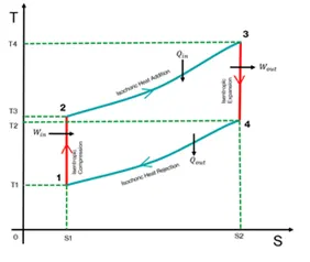
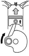
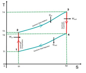
As soon as the piston reaches the BDC, the inlet valve is closed throughout. This means that at this position, piston has inducted some air and has occupied a volume V1 of air inside the cylinder. Now the piston ascends up compressing the charge in an insulated adiabatic environment to a volume V2 whose temperature and pressure are higher than the previous state. This process in the PV diagram is an Isentropic compression process. Please refer to T-S curve for better comparison of Otto Cycle behaviour.

Process 2-3: (Isochoric Heat Addition)

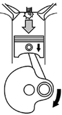
The compressed charge cannot make the temperature high as required for spontaneous burning of charge. Hence an initiation is required by an ignitor which ignites charge & burning takes place. This hydrocarbon compound is rapidly introduced for an exothermic chemical reaction due to which immense increase in temperature & pressure are created. This inturn creates high thermal energy inside the control volume which increases the internal energy of the system. All the above process is so instantaneous that in theory it is said to be processed at a constant volume which is the combustion chamber. This pushes the piston downwards.

Process 3-4: (Isentropic Expansion)

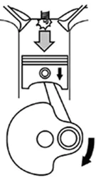
Due to high increase of internal energy, piston is pushed downwards to the BDC, then the temperature & pressure of the charge is reduced, subsequently control volume is increased in an insulated adiabatic environment so that the control volume doesn't loose any heat and get maximum of the work done. This process of is a volume expansion process at isentropic environment.

Process 4-1: (Isochoric Heat Rejection)

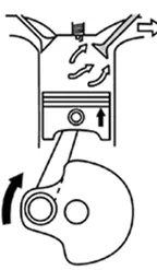
When the piston reaches at BDC, immediately the valve is opened to expel out the pressurised hot air inside the control volume. This process is considered to be so instantaneous in theory that, the heat rejection takes place at a constant volume. Hence this process of heat rejection is Isochoric process.

Process 4-1: (Constant Pressure Scavenging)

After the piston reaches the BDC, due to presence of momentum from the power cycle, the piston tends to move upwards, trying to push the remaining hot air from the control volume. This must eventually increase the control volume pressure but since the exhaust valve is still open, the increase of pressure is compensated by rejection of flux of mass away from the control volume. This is inturn creating a constant pressure condition as same as Air induction process. Hence both these cases in actual condition are cancelled out.

4. Efficiency Calculation for Otto Cycle:

Energy Balancing of Otto Cycle:

Q = ∇U + ∇W

Process	∇U	W (work done)	Q (Heat Added)
1-2	C_v(T2 – T1)	C_v(T1 – T1)	0
2-3	C_v(T3 – T2)	0	C_v(T3 – T2)
3-4	C_v(T4 – T3)	C_v(T3 – T4)	0
4-1	C_v(T1 – T4)	0	C_v(T1 – T4)
	Net ∇U = 0	∑W = ∑Q	∑W = ∑Q

From the above plot, the efficiency of the Otto Cycle can be calculated by T-S diagram:

η = 1- (T4 - T1)/(T3 - T2) which is the ratio of area under the curve of heat rejected by heat added

Expressing efficiency interms of Volumetric Compression Ratio:

Volumetric Compression Ratio (C_R) = (Maximum Volume/Minimum Volume) = V1/V2

We know from isentropic adiabatic condition for Ideal Gas;

PV^γ = constant

For Isothermal process;

PV = RT

Hence (RT/V) *V ^γ = constant

Therefore we can deduce temperature and volume as

T*V^γ= constant

Therefore

T3/T4 = C_R^γ-1

T2/T1 = C_R^γ-1

η = 1-(1/(C_R^γ-1))

5. MATLAB coding for calculation of state variables & PV plot generation for Otto Cycle:

clear all
close all
clc


% State varibales at state point 1....
P1 = 101300;
T1 = 700

% Gamma = Vp/Vc 
gamma = 1.4;
T3 = 2200

% Engine Geometric Parameters
bore = 0.1;
stroke = 0.1;
con_rod = 0.15;
c_r = 12;

% Calculation of Swept Volume(V_S) & Clerance Volume (V_C)
V_S = (pi/4)*(bore^2)*stroke;
V_C = V_S/(c_r -1);

V1 = V_S + V_C;
V2 = V_C;

% State varibales at state point 2...
% P2*V2^gamma = P1*V1^gamma
% P2 = P1*(V1/V2)^gamma
% But V1/V2 = c_r (Compression Ration)
P2 = P1*(c_r)^gamma;

% From Ideal Gas Law:
% PI*VI/T1 = P2*V2/T2
T2 = P2*V2*T1/(P1*V1);
constant_c = P1*V1^gamma;
V_Compression = piston_kinematics(bore,stroke,con_rod,c_r,180,360);
P_Compression = (constant_c)./(V_Compression.^gamma);

% State varibales at state point 3...
V3 = V2;
P3 = P2*(T3/T2);
constant_c = P3*V3^gamma;
V_Expansion = piston_kinematics(bore,stroke,con_rod,c_r,0,180);
P_Expansion = (constant_c)./(V_Expansion.^gamma);

% State varibales at state point 4...
V4 = V1;
P4 = P3*(V3/V4)^gamma;
T4 = P4*V4*T3/(P3*V3);

% Plotting Otto Cycle curves on PV Diagram....
figure(1)
hold on

% Plotting Isentropic Compression curve
plot(V1,P1,'.','color','r')
plot(V_Compression,P_Compression) 
% Plotting Isochoric heat addition curve
plot(V2,P2,'.','color','r')
plot([V2 V3],[P2 P3], 'color','b')
% Plotting Isentropic Expansion curve
plot(V3,P3,'.','color','r')
plot(V_Expansion,P_Expansion)
% Plotting Isochoric heat rejection curve
plot([V4 V1],[P4 P1], 'color','b')
plot(V4,P4,'.','color','r')

% Labeling Axes
xlabel('Volume')
ylabel('Pressure')
grid on

% Efficiency of the Otto Cycle..

% Efficiency calculation using T-S diagram (Expressed interms of Percentage)
Efficiency_TS = (1 - (T4 - T1)/(T3 - T2))*100;

% Efficiency calculation using Compression Ratio relation (Expressed interms of Percentage)
Efficiency_CR = (1 - (1/c_r^(gamma-1)))*100 ;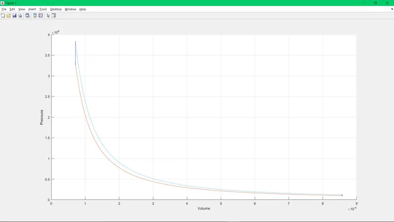

Efficiency using both T-S curve & Volumetric Compression Ratio:

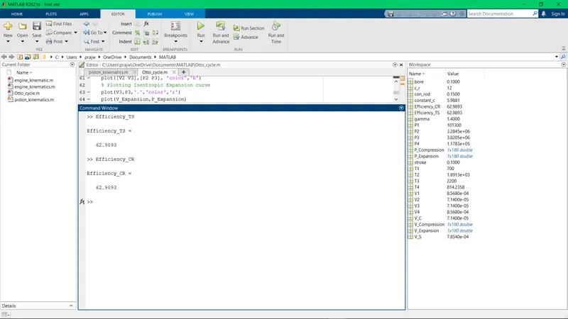
Efficiency of Otto Cycle using both methods were depicted as 62.983%

6. Explaination of Code & Syntax usage Defining Engine Parameters Data

• BORE = 0.1m
• STROKE LENGTH = 0.1m
• CON ROD LENGTH = 0.15m
• COMPRESSION RATIO (c_r) = 12

Assumptions for State Variable Calculations of Otto Cycle

1. P1 = 1 bar
2. T1 = 700 K
3. T3 = 2200K
4. γ = 1.4

Calculation of Max Volume (V1) & Min Volume (V2) using Swept Volume

1. Vswept = (Π/4)*(d^2).(l)
2. V clearance = V swept/(c_r - 1)
3. Total Volume (V1) = V swept + V clearance

From Ideal Gas law for Isentropic & Isochoric processes:

1. PV^γ = constant
2. PV = RT

From these equations and theory above, suitable unknown state variables are calculated.

Volume Trace equation to be calculated since the volume compression & expansion of the Otto cycle depends on Engine Kinematic Parameters

V/V_C = 1+0.5(c_r -1)*{R +1-cos(θ)-(R^2 - (sin(θ)^2)^0.5)

Plotting of Points & Curves

1. a) Initially a plot of points is calculated by calling "plot" function and assigning the state variables of PV diagram
2. b) We can clearly see that after running the program, it fills the points with straight lines which is wrong, as the V compression & expansion for Otto cycle follows the parabolic relation
3. c) Efficiency of Otto cycle is calculated by using formulas:
4. η = 1- (T4 - T1)/(T3 - T2)
5. η = 1-(1/(C_R^γ-1))

Engine Kinematics (Plotting V trace vs Crank Angle)

In order to set the engine kinematic parameters as a function since input data are in huge number, hence a suitable function is done on the name of piston kinematics which is function dependent on Bore,stroke,con rod length, starting crank angle & ending crank angle and then the file is named after the function.

Pin radius R = [Con_rod_length/a]

Volume Traced [V] = 1+0.5(c_r -1)*{R +1-cos(θ)-(R^2 - (sin(θ)^2)^0.5}*(V_C)

For easier coding, the whole equation is divided into three terms as below.

For various angles of crank angle theta, Volume is being traced out to find proper allocation points during piston travel.

Below is the graph obtained after 180 degrees of Crank travel.

% Engine Geometric Parameters
function [V] = piston_kinematics(bore,stroke,con_rod,c_r,start_crank_angle,end_crank_angle)


a = stroke/2;
R = con_rod/a;

V_S = pi/4*bore^2*stroke;
V_C = V_S/(c_r -1);

% Defining Crank Angle variations throughout a stroke

theta = linspace(start_crank_angle,end_crank_angle,180);

% From Engine Geometric Relations of Piston with liner & Con rod relations
% V/V_C = 1+0.5(c_r -1)*{R +1-cosd(theta)-(R^2 - (sind(theta)^2)^0.5)....

term1 = 0.5 *(c_r-1);
term2 = R +1 - cosd(theta);
term3 = (R^2 - sind(theta).^2).^0.5;

V = (1 + term1*(term2 - term3)).*V_C;


end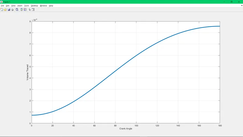

7. Errors commited while coding:

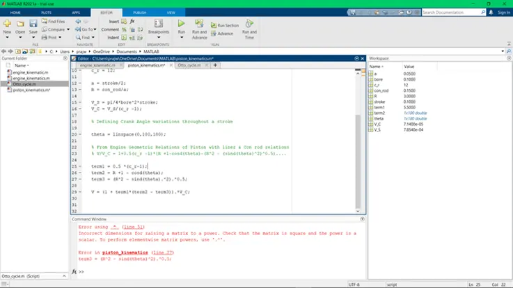
1. a) Incorrect multiplication of Arrayed elements. Did not use a dot product while multiplying the array values.